CSC 458 Data Mining & Predictive Analytics I, Spring 2024, Assignment 2

CSC 458 - Data Mining & Predictive Analytics I, Spring 2024, Assignment 2, Regression.
Due by 11:59 PM on Thursday February 29 via D2L. We will have some work time in class.

You will turn in 2 files by the deadline, with a 10% per day penalty and 0 points after
I go over my solution: CSC458Assn2Small.arff and README.txt with your answers.
Their creation is given in the steps below. I prefer you turn in a .zip folder (no .7z)
containing only those files. You can turn individual files if you don't have a zip utility.

As with all assignments except Python Assignment 4, this is a mixture of two things.
    1. Analysis using stable Weka version 3.8.x. Use this free stable version, not a vendor version.
    2. Answering questions in README.txt

If you are running on a campus PC with the S:\ network drive mounted, clicking:
    s:\ComputerScience\WEKA\WekaWith2GBcampus.bat
    starts Weka 3.8.6. Save your work on a thumb drive or other persistent drive.
    Campus PCs erase what you save on their drives when you log off.
    Many students download Weka 3.8.x and work on their own PCs or laptops.

We are using only 10-fold cross-validation testing in this assignment for
simplicity.

Assignment Background

Here is CSC458S24RegressAssn2Handout.zip containing three files:

    CSC458S24ClassifyAssn1Handout.arff is the Weka Attribute Relation File Format
        dataset with the starting data for Assignment 1. We will use this data briefly.

    CSC458S24RegressAssn2Handout.arff is our related dataset for regression
        analysis in Assignment 2. Regression attempts to predict numeric target
        attribute values in each instance based on non-target attributes that may be
        numeric or nominal.

    README.txt contains questions that you must answer between some steps.

    extractAudioFreqARFF11Feb2024.py is an updated version of
        extractAudioFreqARFF17Oct2023.py used in Assignment 1 for extracting
        data from .wav files.

Please refer to the Assignment 1 handout for background on this audio analysis
    project. In Assignment 2 we are regressing values for the tagged toscgn signal
    gain attribute, with values in the range [0.5, 0.9] on a scale of [0.0, 1.0]
    This attribute is present in both of the handout ARFF files, but we did not use it
    in Assignment 1. It is the only tagged attribute being used in Assignment 2.

A previous semester's handout, recently updated using SciPy's wav file reader and
    fft frequency-domain histogram extraction, serves as a reference.

The main difference between Assignment 1's CSC458S24ClassifyAssn1Handout.arff
    dataset and Assignment 2's CSC458S24RegressAssn2Handout.arff dataset is that,
    whereas the former normalized ampl2 through ampl32 as a fraction of the fundamental
    ampl1 scaled to 1.0, and normalized freq2 through freq32 as a multiple of the
    fundamental frequency of scaled to 1.0, CSC458S24RegressAssn2Handout.arff
    contains neither of these scalings. The amplitude and frequency attributes are
    the values extracted by the wav file read function and the fft frequency-histogram function.
    Figure 1 illustrates that extractAudioFreqARFF11Feb2024.py has extracted the
    fundamental frequency ampl1 as generated by the line "freq = random.randint(100,2000)"
    in the signal generator, with the off-by-1 difference likely due to rounding.

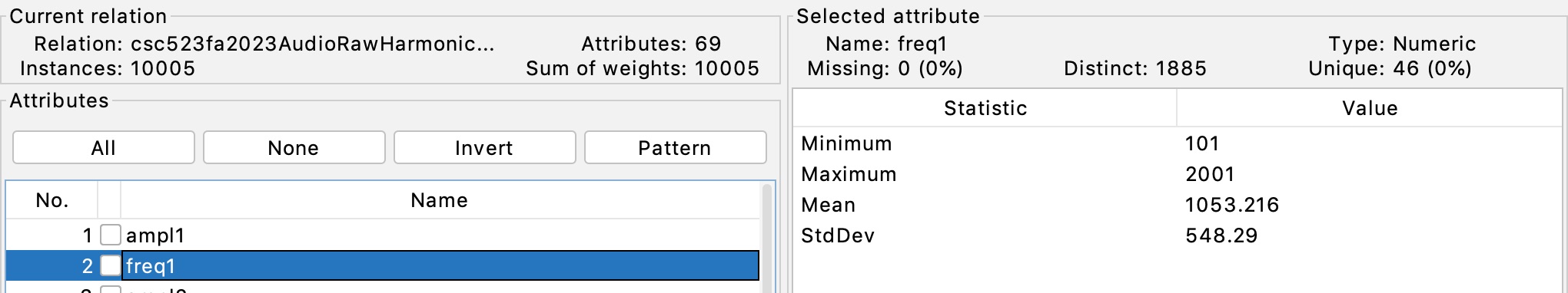
Figure 1: Fundamental frequency ampl1 in range [101.0, 2001.0] per the signal generator

STEP 1: Load CSC458S24RegressAssn2Handout.arff into Weka and Remove tagged attributes
    toosc, tfreq, tnoign and tid as defined in Assignment 1. We will predict signal gain toscgn in the
    range [0.5, 0.9] on a scale of [0.0, 1.0] from non-tagged, non-target attributes. There should be
    65 attributes at this point including toscgn.

NOTE: You can save work-in-progress ARFF files at any time you take a break or want a backup
of your edits.

STEP 2: In Weka's Classify tab run rules -> ZeroR.

README Q1: Paste this part of ZeroR's result in Q1:

ZeroR predicts class value: N.n...Correlation coefficient                 N.nMean absolute error                      N.nRoot mean squared error                  N.nRelative absolute error                N.n      %Root relative squared error            N.n      %Total Number of Instances            10005

README Q2: How does ZeroR arrive at the toscgn value "ZeroR predicts class value: N.n"?
    Use the Weka Preprocess tab to look for your answer. Clicking the ZeroR configuration
    entry line and then More is also helpful.

README Q3: How good is the correlation coefficient of Q1 in predicting toscgn?
    See Evaluating numeric prediction links under Assignment 2 on the course page
    for evaluating testing results.

STEP 3: In Weka's Select Attributes tab run the default Attribute Evaluator of
"CfsSubsetEval -P 1 -E 1" with Search Method set to "BestFirst -D 1 -N5" and
hit Start.

README Q4: Paste this subset of the evaluator's output.

Selected attributes: List and number of attribute indices.
                     ... (paste all lines below "Selected attributes")

README Q5: Given what you know about the fundamental frequency being the
    peak measurement on the left side of the frequency histogram, and the decay rates
    of subsequent ampl measures from Assignment 1 Figure 13, why do you think the
    ampl attributes uncovered in Q4 appear as important for prediction of toscgn?
    Address ampl attributes appearing in Q4.

STEP 4: In Weka's Select Attributes tab select the Attribute Evaluator
"CorrelationAttributeEval", click "yes" for the pop-up Search Method of
Ranker -- it is ranking attribute correlations to toscgn -- and hit Start.

README Q6: Paste the top five results outlined here. How do the first five non-target
attributes pasted in your answer relate to the ranking of STEP 3?

Attribute Evaluator (supervised, Class (numeric): 65 toscgn):
    Correlation Ranking Filter
Ranked attributes:
N.n     n attributeName
N.n     n attributeName
N.n     n attributeName
N.n     n attributeName
N.n     n attributeName

NOTE: The N.n column above is the correlation coefficient of the non-target
attribute to toscgn, the middle n column is the attribute number of this non-target
attribute, followed by its name.

README Q7: In Weka's Classify tab run functions -> SimpleLinearRegression
and paste these output lines. SimpleLinearRegression is the regression counterpart
to classification's OneR, selecting the most strongly correlated non-target attribute
to correlate with toscgn. What attribute does it select, does that selection agree with
the most highly correlated attribute in Q4 and Q6, and has the correlation coefficient
improved over ZeroR?

Linear regression on attributeName...n * attributName + N.n...Correlation coefficient                  N.nMean absolute error                      N.nRoot mean squared error                  N.nRelative absolute error                 N.n %Root relative squared error             N.n %Total Number of Instances            10005

README Q8: In Weka's Classify tab run functions -> LinearRegression
that attempts to use all correlated attributes. Paste this part of its result.

Correlation coefficient                  N.nMean absolute error                      N.nRoot mean squared error                  N.nRelative absolute error                 N.n %Root relative squared error             N.n %Total Number of Instances            10005

Has the correlation coefficient improved over SimpleLinearRegression?
What do you notice about the multipliers in its linear formula?
(Do not paste this formula, just inspect it.)

toscgn =
      n      * attributeName +
      n      * attributeName +

README Q9: In Weka's Classify tab run trees -> M5P
that attempts to use all correlated attributes. The M5P decision
tree divides non-linear data relationships into leaves that
are approximations of linear relationships in the form of
linear expressions. Has the correlation coefficient improved over
LinearRegression? How good is it?
What do you notice about the multipliers in its linear formulas?
What do you notice about the magnitude of values in its decision
tree?

Paste this part of its result.

Correlation coefficient                  N.n
Mean absolute error                      N.n
Root mean squared error                  N.n
Relative absolute error                 N.n %
Root relative squared error             N.n %
Total Number of Instances            10005

NOTE: There are two problems with this dataset. First, the magnitude of the
correlated non-target attribute values are very high, leading to the apparent
multipliers in the above linear expressions. Second, there are too many attributes.

STEP 5: Remove all attributes except the top 2 "Selected attributes" for Q4
plus toscgn. There are only 3 attributes now.

README Q10: In Weka's Classify tab run trees -> M5P and paste
the following out. How does CC compare to that of Q9?
What do you notice about the multipliers in its linear formulas?

Paste this part of its result.

Correlation coefficient                  N.n
Mean absolute error                      N.n
Root mean squared error                  N.n
Relative absolute error                 N.n %
Root relative squared error             N.n %
Total Number of Instances            10005

STEP 6: In Weka's Preprocess tab run Filter -> unsupervised -> attribute -> MathExpression
with the default formula "(A-MIN)/(MAX-MIN)". Unlike AddExpression which creates
a new named derived attribute, MathExpression with default settings applies its formula
to every non-target attribute in the dataset. Unlike Assignment 1 where amplitudes
and frequencies were normalized against the amplitude and frequency of the
fundamental frequency, "(A-MIN)/(MAX-MIN)" normalizes each non-target attribute
as a fraction of its respective distance between that attribute's individual minimum and
maximum values. This is a within-attribute, across-all-instances normalization, not a
cross-attribute as in Assignment 1's dataset.
Make sure to Apply and inspect in Preprocess that the two non-target attributes have
been mapped, linearly, into the range [0.0, 1.0], and that toscgn remains in the range
[0.5, 0.9]. We want predictions in toscgn application terms.

(SIDE NOTES: 1. After prepping and reviewing this assignment, I found that
SciPy's fft function has a parameter called norm that when changed from the default
"backward" to "forward" value, brings the range of histogram values down into a lower
range that makes linear expression multipliers more visible in Weka without affecting
accuracy of predictions. 2. The default MathExpression formula above gives identical
results to Weka's Normalize attribute filter. 3. In some assignments we use the
Normalize filter, not to make multipliers more visible in Weka, but to put them
on the same within-attribute [0.0, 1.0] range so we can compare their multipliers
for improtance. 4. I decided to leave the initial fft result in place in order to support practice
using a Weka filter.)

SAVE this 3-attribute dataset after applying MathExpression as CSC458Assn2Small.arff
and turn it into D2L with your README.txt file by the deadline.

README Q11: In Weka's Classify tab run trees -> M5P and paste
the following output. How do CC, MAE, and RMSE compare to those of Q10?
What do you notice about the multipliers in its linear formulas?
Also, how do the MAE (mean absolute error) and RMSE (root mean squared error)
measures compare to the toscgn range of values [0.5, 0.9] and its mean?

Paste this part of its result.

Number of Rules : nn
...
Correlation coefficient                  N.n
Mean absolute error                      N.n
Root mean squared error                  N.n
Relative absolute error                 N.n %
Root relative squared error             N.n %
Total Number of Instances            10005

README Q12: In Weka's Classify tab select rules -> DecisionTable, go into its
configuration settings and set displayRules to true, and run it. How many rows
of rules are there, and how many linear formulas ("Number of Rules) in M5P for Q11?
How do the complexity of Q11's and Q12's models compare? How do their CCs compare?

Paste this part of its result.

Number of Rules : nn
...
Correlation coefficient                  N.n
Mean absolute error                      N.n
Root mean squared error                  N.n
Relative absolute error                 N.n %
Root relative squared error             N.n %
Total Number of Instances            10005
Number of training instances: 10005

README Q13: In Weka's Classify tab select trees -> M5P,
go into its configuration settings and set minNumInstances to
1000. This increase will put more instances at each leaf than
in the default value for minNumInstances, resulting in more
shallow trees that are possibly easier to read.
How many linear formulas ("Number of Rules) in M5P for Q13 compared to Q11?
How do the complexity of Q11's and Q13's models compare?
How do their CCs compare?

Paste this part of its result.

Number of Rules : n
...
Correlation coefficient                  N.n
Mean absolute error                      N.n
Root mean squared error                  N.n
Relative absolute error                 N.n %
Root relative squared error             N.n %
Total Number of Instances            10005

README Q14: Load Assignment 1's CSC458S24ClassifyAssn1Handout.arff into Weka,
remove remove tagged attributes toosc, tfreq, tnoign and tid. Run M5P with the
minNumInstances parameter set to the default value of 4. Next remove all attributes
except the top 2 "Selected attributes" for Q4 plus toscgn. There are only 3 attributes now.
Run M5P again. What are their CC values? How do these CCs of M5P using
CSC458S24ClassifyAssn1Handout.arff compare to the earlier M5P runs with
CSC458S24RegressAssn2Handout.arff and CSC458Assn2Small.arff? /
Why are these CSC458S24ClassifyAssn1Handout.arff results so substantially different?
Think about the differences between CSC458S24ClassifyAssn1Handout.arff's
versus CSC458S24RegressAssn2Handout.arff's values for non-target attributes.
Also, look at the attributes in Q14's decision trees compared to the earlier
M5P trees using CSC458S24RegressAssn2Handout.arff's data.

Correlation coefficient                  N.n    (for the 65-attribute dataset after removing the other tagged attributes)

Correlation coefficient                  N.n    (for the 3-attribute dataset after removing all but 3 attributes))

README Q15: These are the remaining 6.6% for turning in a correct CSC458Assn2Small.arff file.