CSC 458 - Data
Mining & Predictive Analytics I, Spring 2024, Assignment 1, Classification.
Due by 11:59 PM on Thursday February 15 via D2L. We will have
some work time in class.
You will turn in 6 files by the deadline, with a 10% per day
penalty and 0 points after
I go over my solution: CSC458S24ClassifyAssn1Turnin.arff,
handouttrain.arff,
handouttest.arff,
randomtrain.arff,
randomtest.arff,
and README.txt
with your
answers.
Their creation is given in the steps below. I prefer you
turn in a .zip folder (no .7z)
containing only those files. You can turn individual files
if you don't have a zip utility.
As with all assignments except Python Assignment 4,
this is a mixture of two things.
1. Analysis using stable Weka
version 3.8.x. Use this free stable version, not a vendor
version.
2. Answering questions in
README.c458s24assn1.txt
If you are running on a campus PC with the S:\ network drive
mounted, clicking:
s:\ComputerScience\WEKA\WekaWith2GBcampus.bat
starts Weka 3.8.6. Save your work on a thumb
drive or other persistent drive.
Campus PCs erase what you save on their drives
when you log off.
Many students download Weka 3.8.x and work on
their own PCs or laptops.
Assignment Background
Here is CSC458S24ClassifyAssn1Handout.zip
containing three files:
CSC458S24ClassifyAssn1Handout.arff is
the Weka Attribute Relation File Format
dataset with the starting
data.
README.txt contains questions that you
must answer between some steps.
extractAudioFreqARFF17Oct2023.py is my
Python file used to extract data from .wav files.
This is included in the handout so we can go
over example Python scfipts before Assignment 4.
Our application domain is audio signal analysis using data that I
generated
I have made changes to the analyses so it will not be a repeat of
a CSC523 project.
The dataset remains the same, but the data preparation &
analyses differ.
Figure 1 shows a generated 1000 Hz. (cycles per second) audio
waveform in the time domain.
This is the third waveform whose data appears in your handout ARFF
file.
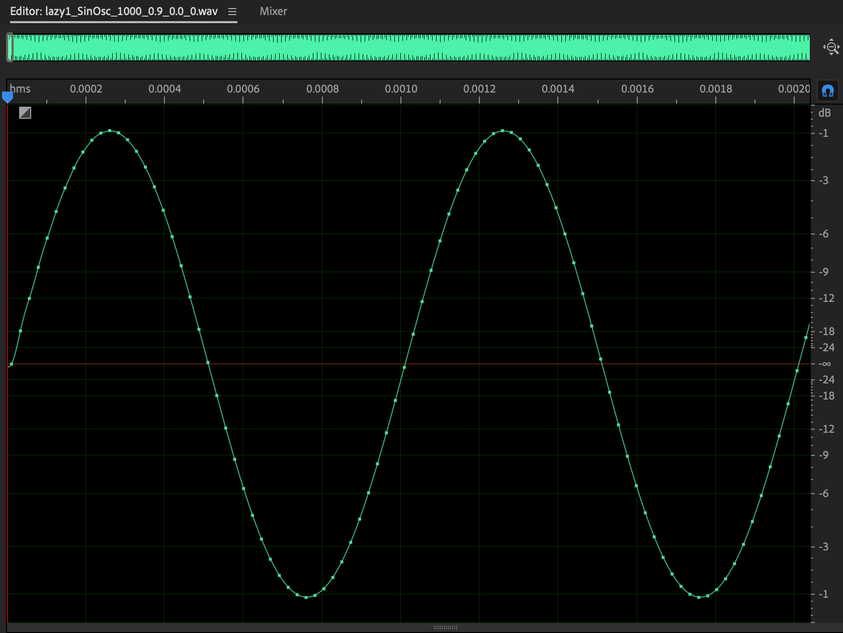 Figure 1: 1000 Hz sin wave with gain of 0.9 on
scale [0.0, 1.0] with white noise of 0.
Figure 1: 1000 Hz sin wave with gain of 0.9 on
scale [0.0, 1.0] with white noise of 0.
Here
is what this .wav file sounds like (TURN DOWN YOUR AUDIO!).
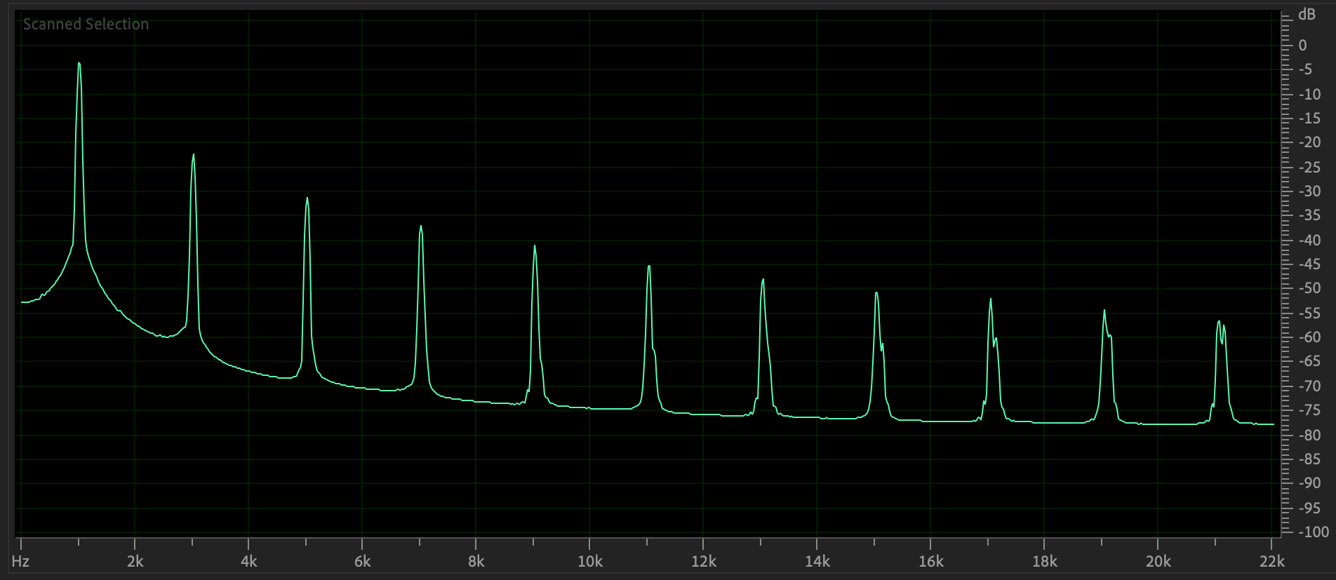
Figure 2 shows the frequency domain plot of the same .wav file.
These plots act like histograms of frequency components of their
signals.
The decibel scale on the right of these plots is logarithmic.
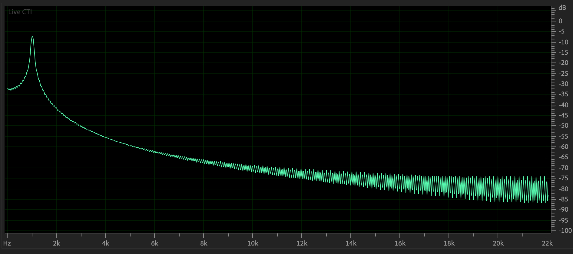
Figure 2: Frequency domain plot
of Figure 1's waveform.
Note that the sin wave is primarily its fundamental frequency at
1000 Hz.
Figures 3 and 4 show the time and frequency domain plots of a 1000
Hz.
pulse wave with a gain of 0.9 and white noise of 0.0, the first
instance
in your starting ARFF file.
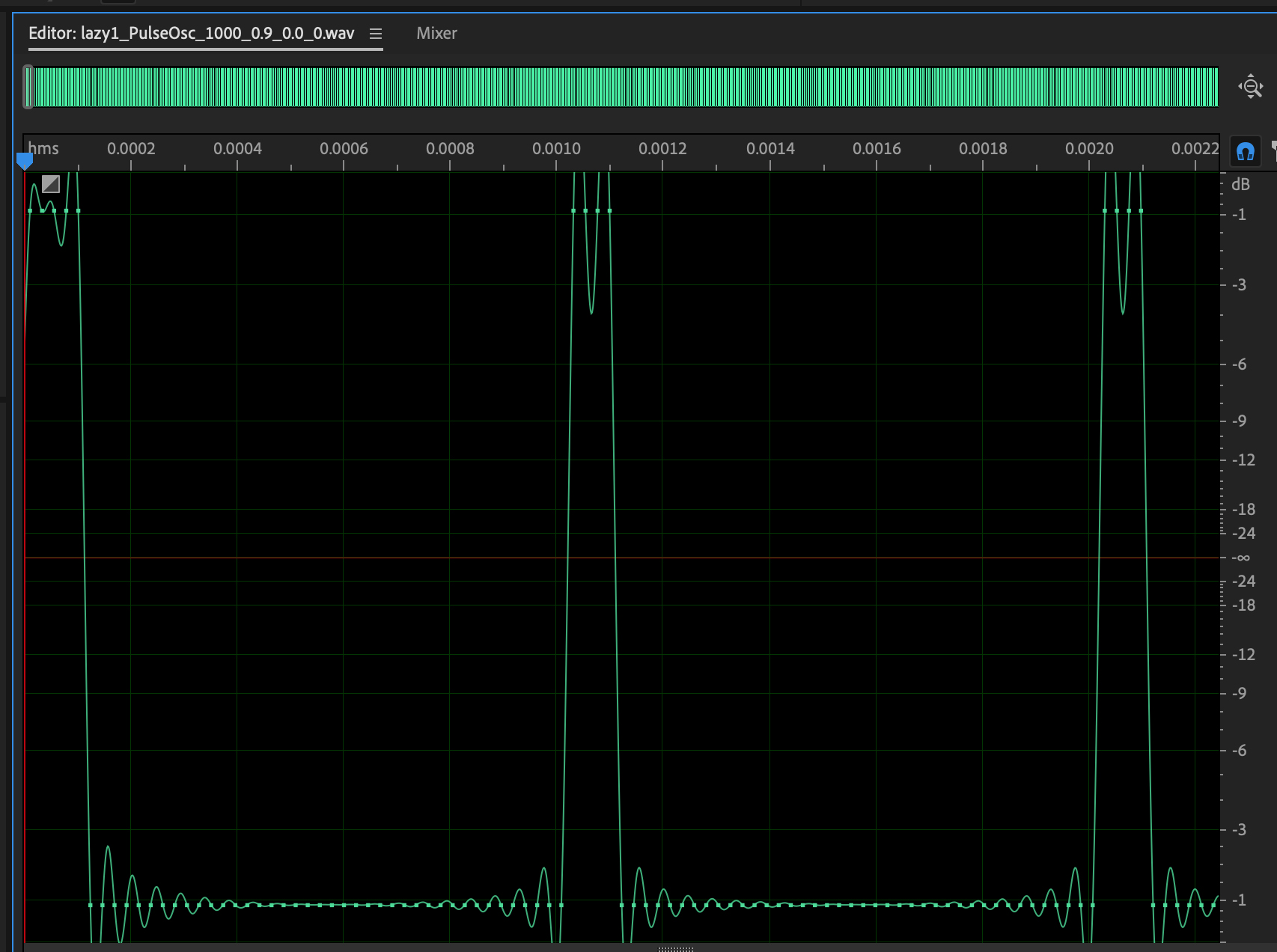
Figure 3: 1000 Hz pulse wave,
gain=0.9, white noise=0.0.
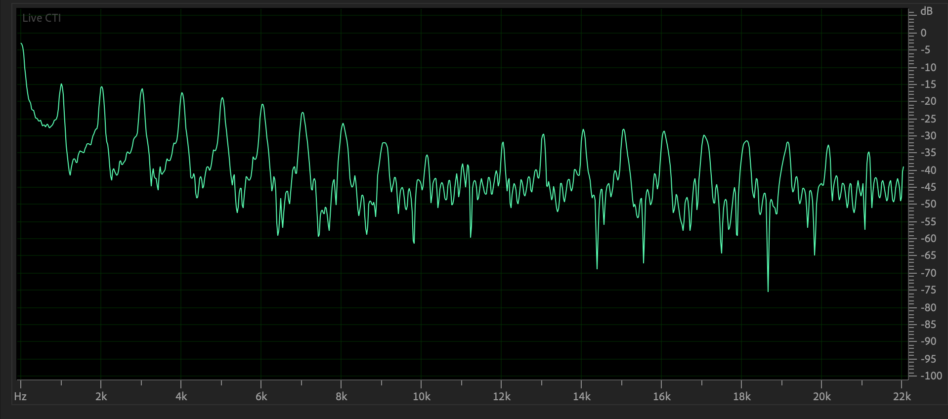
Figure 4:
Frequency domain plot of Figure 3's waveform.
Note that the pulse contains peaks at both even & odd
multiples of the 1000 Hz. fundamental.
Unlike others, it has some low frequency noise. Here
is its sound (CAREFUL!).
Figures 5 and 6 show the time and
frequency domain plots of a 1000 Hz.
sawtooth wave with a gain of 0.9 and white noise of 0.0, the
second instance
in your starting ARFF file.
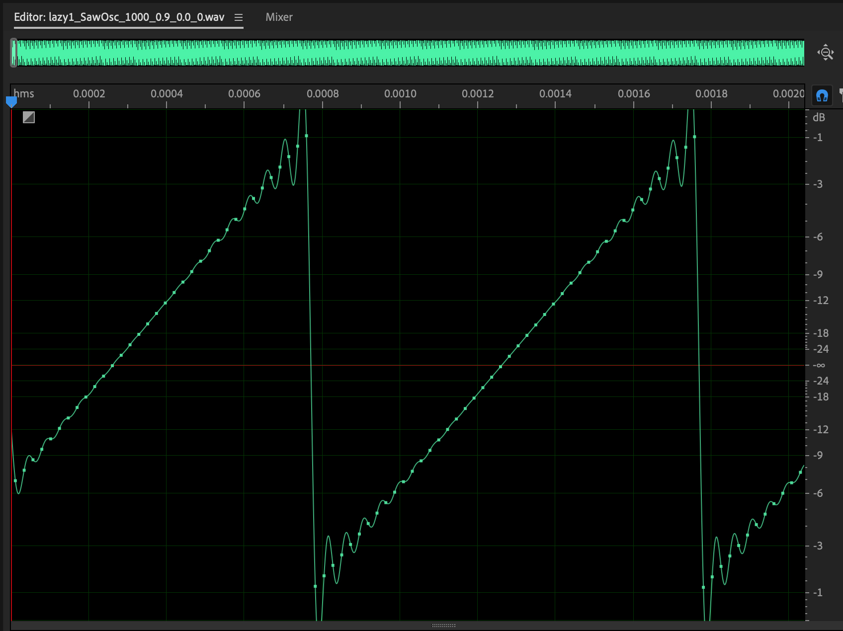
Figure 5:
1000 Hz sawtooth wave, gain=0.9, white noise=0.0.
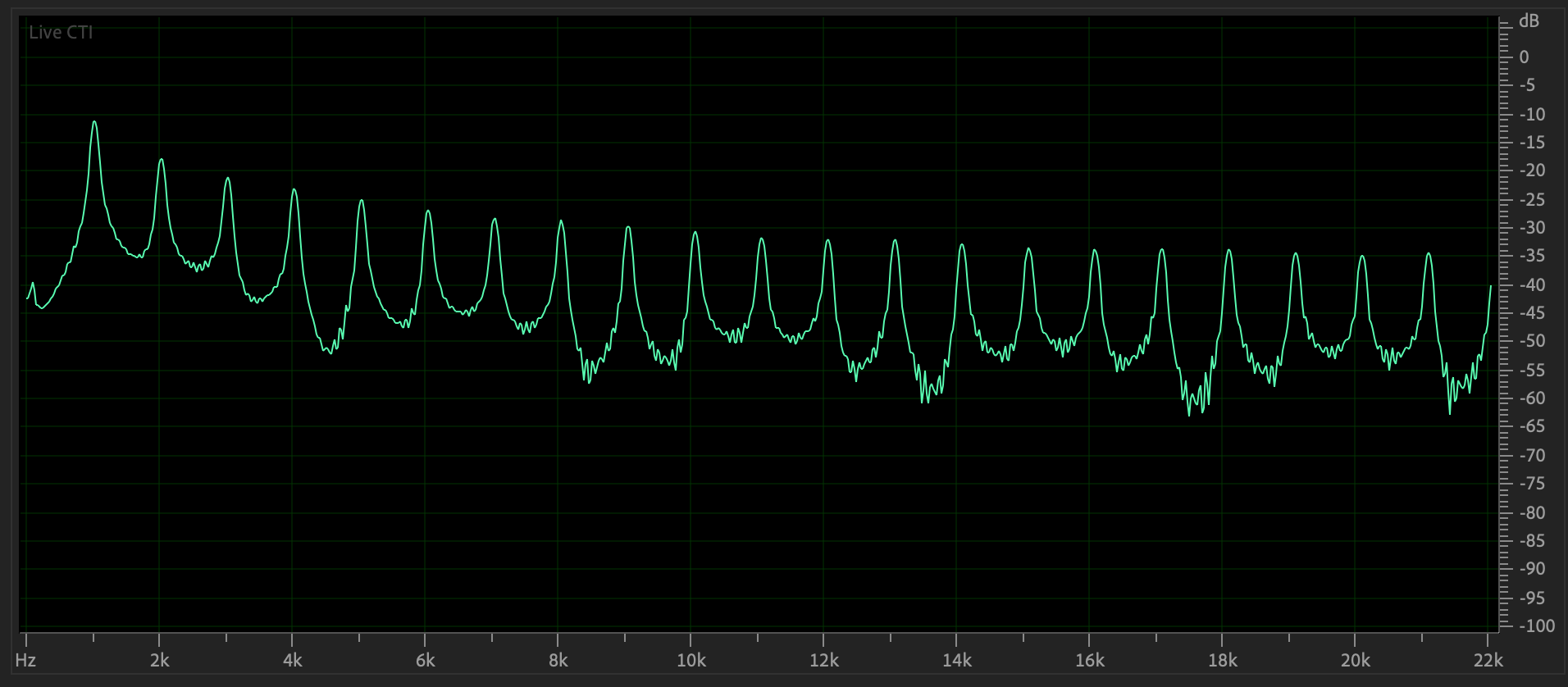
Figure
6: Frequency domain plot of Figure 5's waveform.
Sawtooth also contains peaks at both even &
odd multiples of the 1000 Hz. fundamental,
but peaks decay faster than the pulse. Here
is its sound (CAREFUL!).
Figures 7 and 8 show
the time and frequency domain plots of a 1000 Hz.
square wave with a gain of 0.9 and white noise of 0.0, the
fourth instance
in your starting ARFF file.
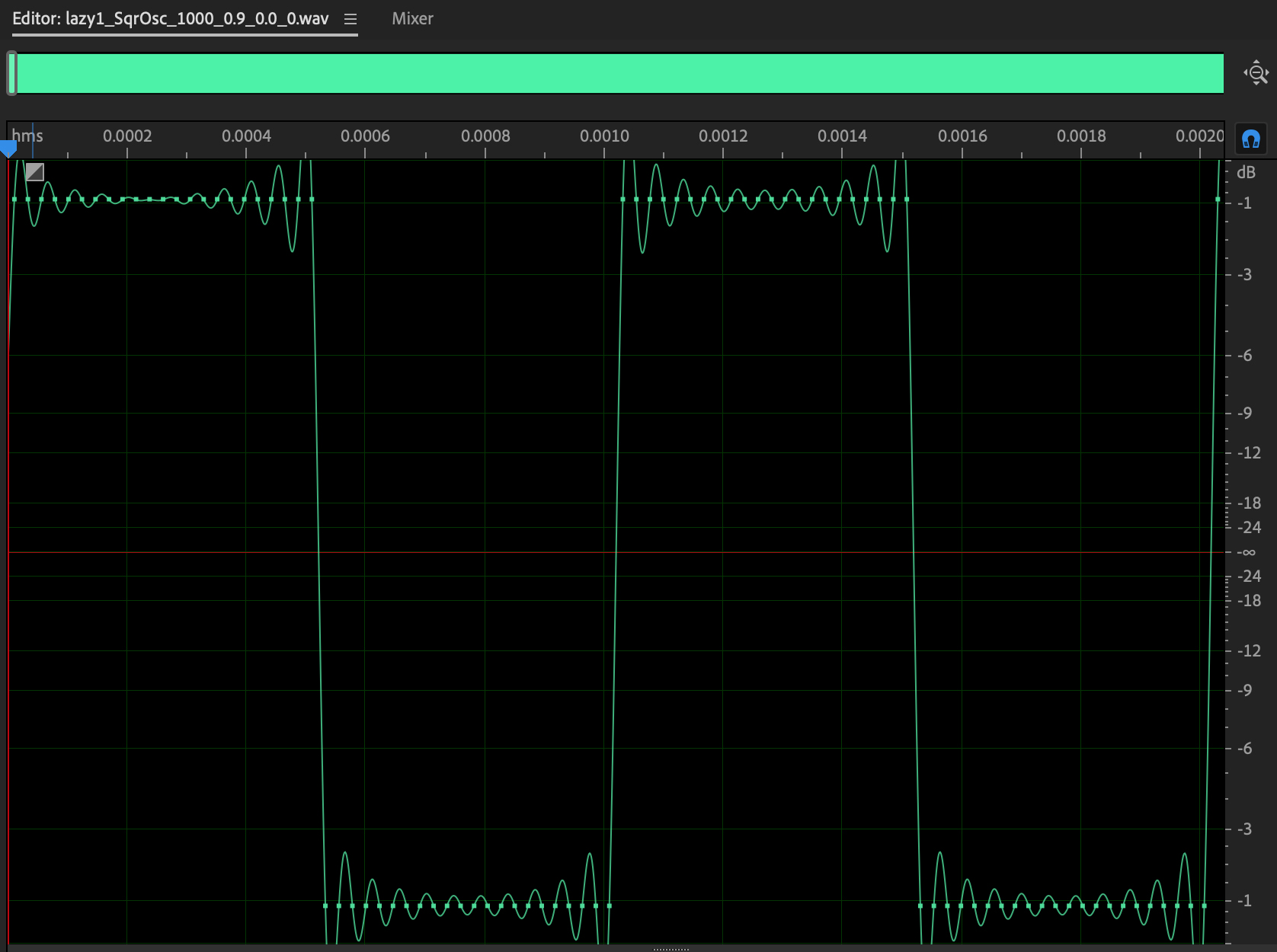
Figure 7: 1000 Hz
square wave, gain=0.9, white noise=0.0.
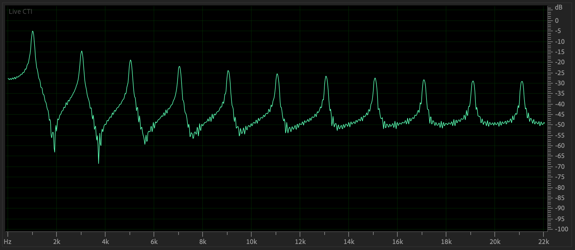
Figure 8: Frequency domain plot
of Figure 7's waveform.
Square waves contain
peaks only at odd multiples of the 1000 Hz. fundamental,
Here
is its sound (CAREFUL!).
Figures
9 and 10 show the time and frequency domain plots of a 1000
Hz.
triangle wave with a gain of 0.9 and white noise of 0.0, the
fifth instance
in your starting ARFF file.
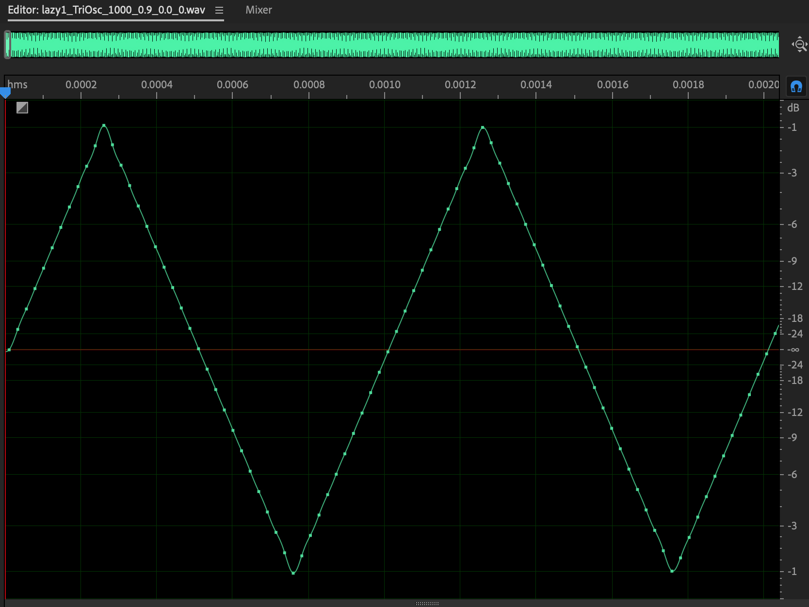
Figure 9:
1000 Hz triangle wave, gain=0.9, white
noise=0.0.
Figure
10: Frequency domain plot of Figure 9's
waveform.
Triangle also contains peaks at
only odd multiples of the 1000 Hz. fundamental,
but peaks decay faster than the square. Here
is its sound (CAREFUL!).
Figures
11 and 12 show the time and frequency domain plots of a 1380
Hz.
sin wave with a gain of 0.718 and white noise of 0.228. This
.wav has data in
one of the rows of your ARFF file.
We will regress white noise levels in a later assignment. In
this assignment
we are classifying waveform type.
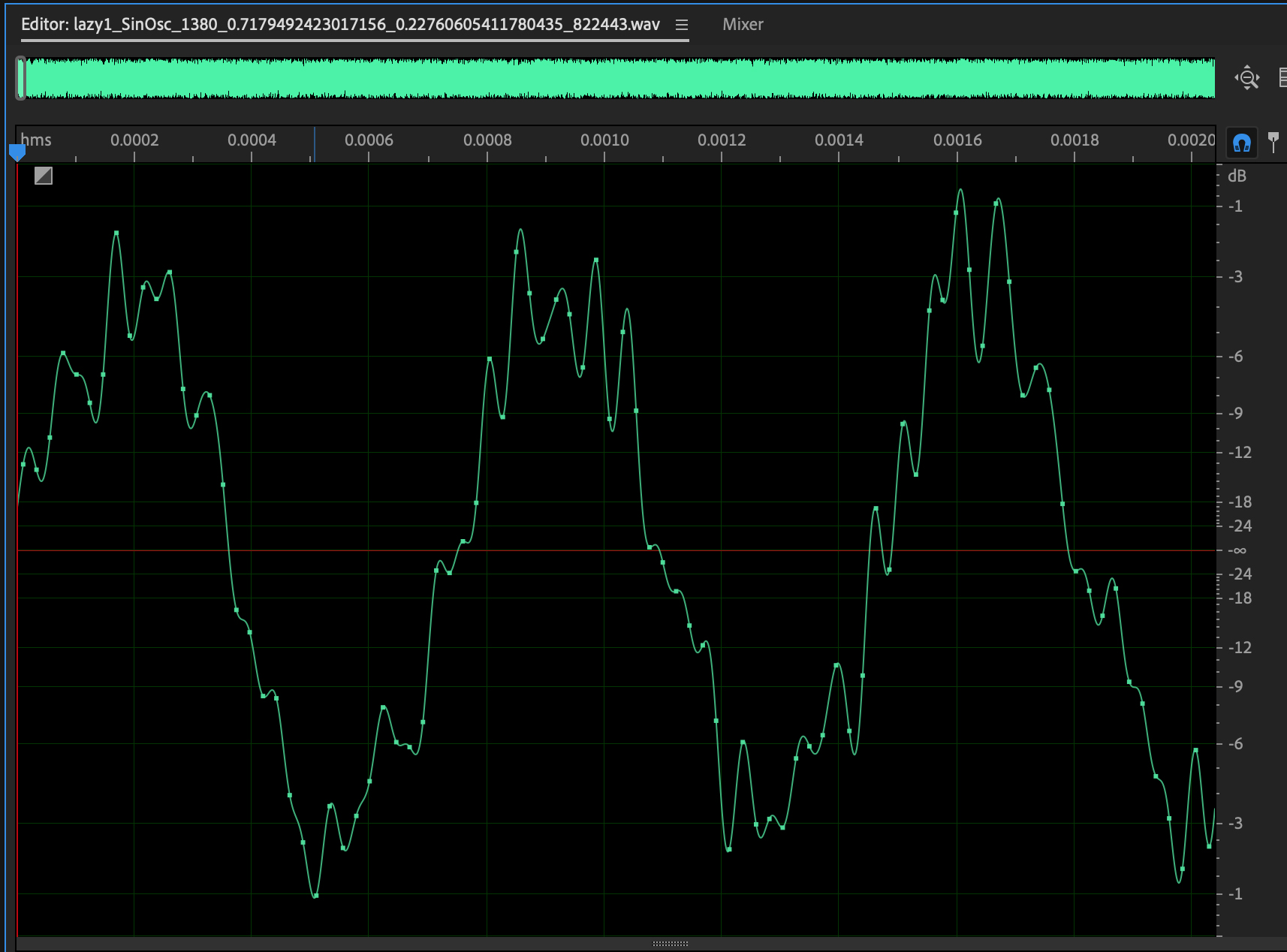
Figure 11: 1380 Hz sin wave,
gain=0.718, white noise=0.228.
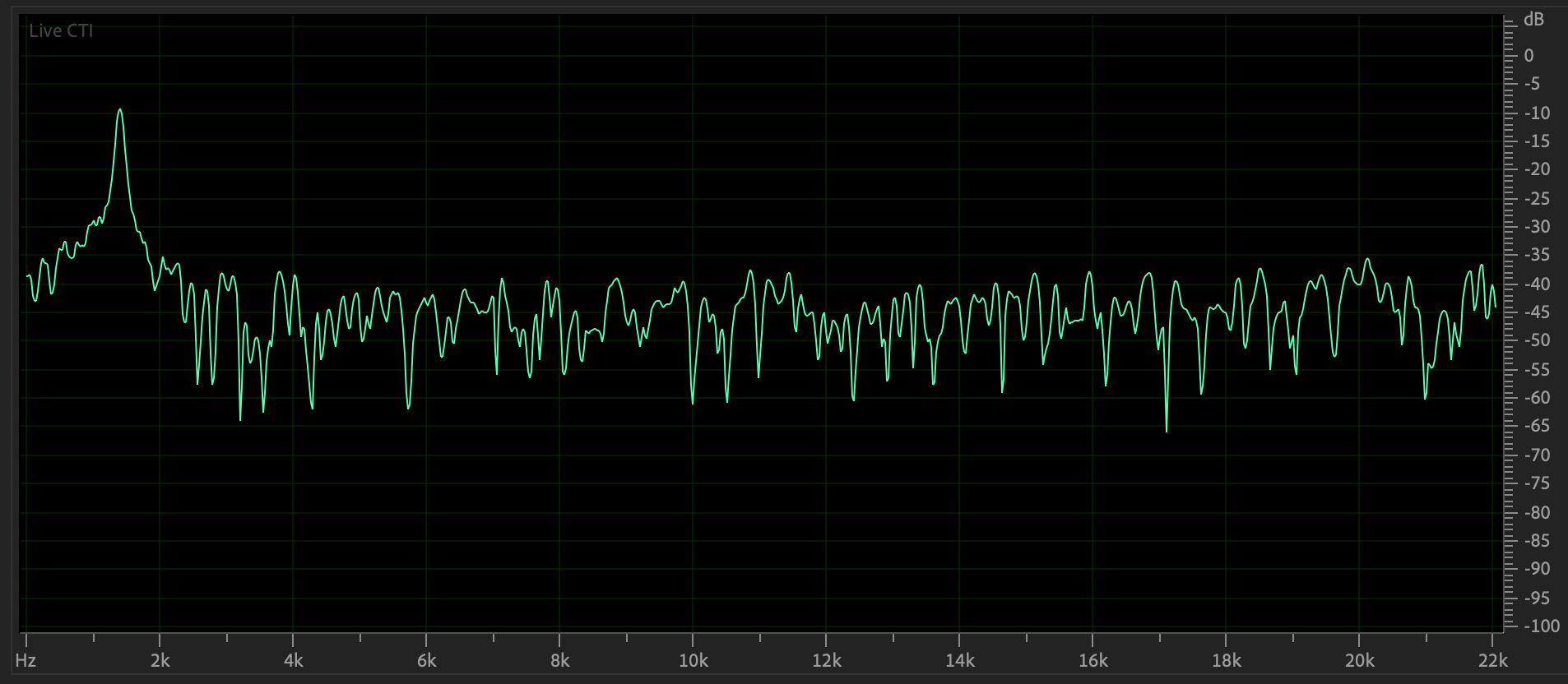
Figure 12:
Frequency domain plot of Figure 11's
waveform.
Signal gain levels range from 0.5 to 0.75 in this
dataset except for
the 0-noise 5 reference examples which have signal gain=0.9 on
the scale of [0.0, 1.0]. White noise gains vary from 0.1 to 0.25
except for those 5 0-noise instances.
Here are the data attributes (CSV columns) in your handout ARFF
file.
@relation csc523fa2023AudioHarmonicData_32
@attribute ampl1 numeric
Amplitude of fundamental freq normalized to 1.0
@attribute freq1 numeric
Frequency of fundamental normalized
to 1.0
@attribute ampl2 numeric
Second strongest amplitude as a fraction of ampl1.
@attribute freq2
numeric
Frequency of ampl2 as a multiple of freq1.
@attribute ampl3 numeric
@attribute freq3 numeric
@attribute ampl4 numeric
@attribute freq4 numeric
... (ampl5 through freq31 elided).
@attribute ampl32 numeric
@attribute freq32 numeric
@attribute toosc
{PulseOsc,SawOsc,SinOsc,SqrOsc,TriOsc} Tagged
waveform type
@attribute tfreq numeric
Tagged fundamental frequency
@attribute toscgn numeric
Tagged signal gain
@attribute tnoign numeric
Tagged white noise gain
@attribute tid numeric
Tagged instance
ID
@data
CSV instance-per-row data instances (rows) follow
Figure 13 shows the ampl1 through freq4
and the tagged toosc target attribute values
of the first 10 instances in your handout ARFF file. Note the even
and odd harmonics
in the pulse and sawtooth waves, with faster amplitude decay in
the latter, and the
odd harmonics in the square and triangle waves, with faster amplitude decay in the latter.
The sin wave is only a fundamental plus some very minor noise.
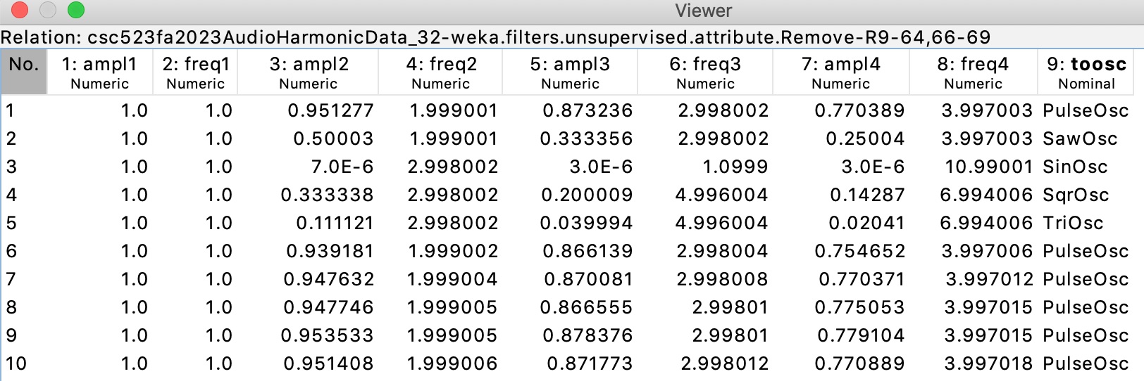
Figure
13: The first ten instances in CSC458S24ClassifyAssn1Handout.arff.
extractAudioFreqARFF17Oct2023.py extracts .wave file audio
data into
CSC458S24ClassifyAssn1Handout.arff.
YOUR WORK ASSIGNMENT.
Any answers to README questions must go into the handout
README.txt file.
STEP 1: Load CSC458S24ClassifyAssn1Handout.arff
into Weka.
If you use Weka's editor, before careful not to reorder instances
until instructed to do so.
STEP 2: After noting how many attributes there are in the
Weka Preprocess tab,
run the following filter that I will demo in class. Figure 14
shows a screen shot of this step.
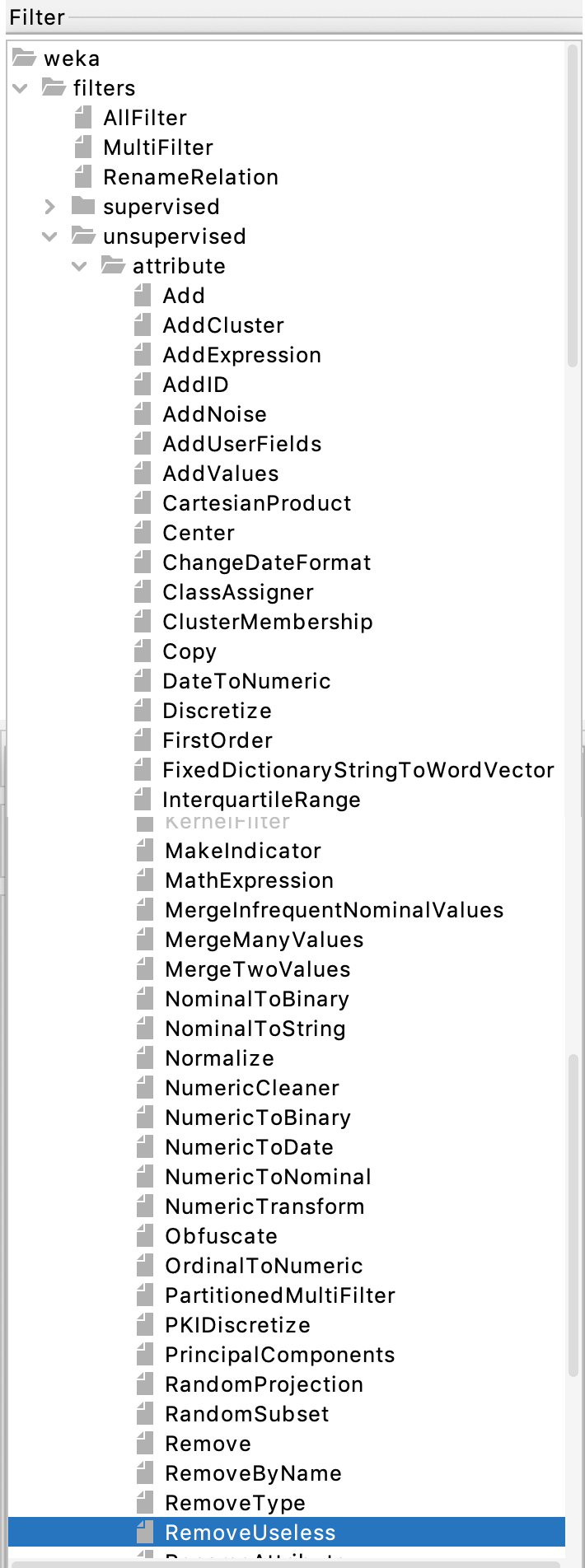
Figure 14: Filter -> unsupervised -> attribute
RemoveUseless
Supervised filters attempt to correlate changes to the target
attribute,
toosc in this case. Unsupervised filters just make the entered
changes.
Hit Apply in the Weka Preprocess tab to run this filter.
README Q1: What attributes did RemoveUseless remove?
Why do you think it removed these?
STEP 3: Go into Weka's Edit window and sort
instances in ascending
order on the ampl2 column header. Observe the
minimum value comes
to the top. Click OK to save this change.
Manually delete tagged attributes tfreq, toscgn, tnoign,
and tid.
This step leaves 63 attributes.
We will classify the remaining tagged target attribute toosc.
Save this dataset as CSC458S24ClassifyAssn1Turnin.arff.
You will turn that in along with your README.txt file with
answers
and 4 additional ARRF files that you will create: handouttrain.arff,
handouttest.arff,
randomtrain.arff,
and randomtest.arff.
Initial testing uses 10-fold cross-validation, which means
training models
on 9/10ths of randomly selected instances, testing on the
remaining tenth,
then repeating the process 9 more times, and integrating the
results.
In later steps we will use different training and testing portions
of
CSC458S24ClassifyAssn1Turnin.arff.
STEP 4: In Weka's Classify tab run Classifier ->
rules -> ZeroR.
README Q2: Copy and paste the following Weka output.
You must use control-C to copy.
Correctly Classified
Instances N
N.n %
Incorrectly Classified
Instances N
N.n %
Kappa
statistic
N.n
Mean absolute
error
N.n
Root mean squared
error
N.n
Relative absolute
error
N %
Root relative squared
error
N %
Total Number of
Instances
N
=== Confusion Matrix ===
a b c
d e <-- classified as
N N N
N N | a = PulseOsc
N N N
N N | b = SawOsc
N N N
N N | c = SinOsc
N N N
N N | d = SqrOsc
N N N
N N | e = TriOsc
README Q3: What percentage of the 10,005 instances are
correctly classified?
Given the number of distinct waveform types, how much better is
this percentage
than a random guess?
Note the kappa
value that we will go over in class. It is our primary
measure of accuracy
in this assignment.
STEP 5: In Weka's Classify
tab run Classifier -> rules -> OneR.
README Q4: Copy and paste the following Weka output.
=== Classifier model (full training set) ===
ampl2:
SHOW THE FULL OneR rule here.
(N/10005 instances correct)
Correctly
Classified
Instances N
N.n %
Incorrectly Classified
Instances N
N.n %
Kappa
statistic
N.n
Mean absolute
error
N.n
Root mean squared
error
N.n
Relative absolute
error
N %
Root relative squared
error
N %
Total Number of
Instances
N
=== Confusion Matrix ===
a b c
d e <-- classified as
N N N
N N | a = PulseOsc
N N N
N N | b = SawOsc
N N N
N N | c = SinOsc
N N N
N N | d = SqrOsc
N N N
N N | e = TriOsc
README Q5: How well did the OneR model do in terms of %
correct and Kappa?
README Q6: What non-target attribute appearing in "Classifier
model" above
did Weka use to classify toosc?
README Q7: In terms of the paragraph preceding Figure 13 in the
handout,
why do you think OneR selected this attribute?
STEP
6: In Weka's Classify tab run Classifier ->
trees -> J48.
README Q8: Copy and paste the following Weka output.
J48 pruned tree
------------------
SHOW THE DECISION TREE in README
Number of Leaves : N
Size of the tree : N
Correctly Classified
Instances N
N.n %
Incorrectly Classified
Instances N
N.n %
Kappa
statistic
N.n
Mean absolute
error
N.n
Root mean squared
error
N.n
Relative absolute
error
N %
Root relative squared
error
N %
Total Number of
Instances
N
=== Confusion Matrix ===
a b
c d e
<-- classified as
N N
N N N
| a = PulseOsc
N N
N N N
| b = SawOsc
N N
N N N
| c = SinOsc
N N
N N N
| d = SqrOsc
N N
N N N
| e = TriOsc
README Q9: How did J48 do in terms of kappa, and
how well
did it do in terms of kappa compared to OneR in Q4 and
Q5?
README Q10: What non-target attributes appear in
J48's "J48
pruned tree"
decision tree. How does this tree compare with OneR's
rule in terms of
intelligibility, i.e., which one is easier to
understand.
Decision tree builders use information
entropy to decide the binary split points.
The concept of Minimal Description Length (MDL) refers
to finding the most
intelligible model (easy to understand) that is no more
than 10% less
accurate (in terms of kappa for classification) than the
most accurate
model that is presumably less intelligible. The 10%
threshold is my rule-of-thumb.
README Q11: Which of these two models above,
OneR's rule versus J48's tree,
exhibits the MDL so far? Justify your answer.
STEP 7: Take a look at J48's Confusion matrix of
Q8. Each row shows how
instances should have been classified, and each column
shows how they were classified.
A perfect diagonal with all entries off the diagonal
being zeros is perfect.
README Q12: How many instances in J48's
confusion matrix were misclassified.
Describe each non-0 entry that is off the diagonal in
terms of:
Number incorrect at that spot, what it should have been,
what it was classified as.
STEP 8: Run the filter Filter ->
unsupervised -> instance -> RemovePercentage
with the default percentage of 50% and invertSelection
set to false.
This remove the first 50% of the instances.
Apply this filter and note the number of
remaining instances.
Save this 50% dataset as handouttest.arff.
STEP 9: Execute Undo once and verify that all
10,005 instances have returned.
Run the filter Filter -> unsupervised
-> instance -> RemovePercentage
with the default percentage of 50% and
invertSelection set to true this
time.
This
remove the last 50% of the
instances.
Apply this filter and
note the number of remaining
instances.
Save this 50% dataset as handouttrain.arff.
STEP 10: With handouttrain.arff
still in Weka, go to the Classify tab and
set
Supplied test set to handouttest.arff.
We are using handouttrain.arff
for training models and
handouttest.arff
for testing them with a different dataset to
avoid testing on the training data.
Run OneR and J48 on this training / testing
configuration.
README Q13: How do OneR and J48 do in
terms of % correct and kappa
compared to 10-fold cross validation in Q4
and Q8?
STEP 11: Load CSC458S24ClassifyAssn1Turnin.arff
back into Weka.
Run Filter ->
unsupervised -> instance ->
Randomize
with a default seed of 42. Apply this filter ONLY
ONCE to shuffle the instance order.
STEP 12: Run the filter Filter -> unsupervised
-> instance -> RemovePercentage
with the default percentage of 50% and
invertSelection set to false.
As in STEP 8, his remove the first 50% of
the instances.
Apply this filter and note the number
of remaining instances.
Save this 50% dataset as randomtest.arff.
STEP 13: Execute
Undo once and verify that all
10,005 instances have returned.
Run the
filter
Filter ->
unsupervised
-> instance
->
RemovePercentage
with the default
percentage of 50%
and invertSelection
set to true
this time.
This
remove the
last 50% of
the instances.
Apply
this filter
and note the
number of
remaining
instances.
Save this
50% dataset as randomtrain.arff.
STEP
14: With randomtrain.arff
still in Weka,
go to the
Classify tab
and set
Supplied test
set to randomtest.arff.
We are using randomtrain.arff
for training
models and
randomtest.arff
for testing
them with a
different
dataset to
avoid testing
on the
training data.
Run OneR and
J48 on this
training /
testing
configuration.
README Q14:
How do OneR
and J48 do in
terms of %
correct and
kappa
compared to 10-fold
cross
validation
those test
results in
Q13
that used handouttrain.arff
and handouttest.arff?
(Note: Neither
Q13 nor Q14
uses
cross-validation.
That was a
wording
mistake,
please ignore
it.)
README Q15: What accounts in the differences in OneR's
and J48's kappa values in Q14
compared to Q13? To figure this out, load handouttrain.arff,
handouttest.arff,
randomtrain.arff,
and randomtest.arff,
one at a time, into the Preprocess tab and
look at the toosc distributions by clicking that
attribute and looking at its distribution
in the Selected attribute panel in the upper right of
the Preprocess tab.
Each of Q1 through Q15 is worth 6%, giving 90%.
Each file CSC458S24ClassifyAssn1Turnin.arff,
handouttrain.arff,
handouttest.arff,
randomtrain.arff,
and randomtest.arff
is worth 2% each if correct.
Make sure to turn in all 5 ARFF files + README.txt with answers.
You can zip a folder with these 6 files or turn them into D2L
individually.