CSC 558, Spring 2023, Assignment 3

CSC 558 - Predictive Analytics II, Spring 2023, Assignment 3 on time series.

Assignment 3 due by 11:59 PM on Sunday April 9 via D2L Assignment 3

Answer to a March 29 question added here on March 30:

These questions came up after most students left Zoom. For SS_All using the monthly data my Q2 for M5P looks like this (These are in the last 15 minutes of the zoom recording):

Correlation coefficient 0.699 Mean absolute error 688.5367Root mean squared error 1240.3141Relative absolute error 52.7569 %Root relative squared error 71.2516 %Total Number of Instances 229

To figure out importance of the attributes in the decision tree, the ones closest to the left are the most important. They are near the root and split the decision subspace below them, ideally in half. For the above tree, the most important attributes are:

HMtempC_median (0 steps from left)

HMtempC_mean

wndNW

HMtempC_mean_td

There are only 4 in the above tree. Also, if you get a tie with respect to depth in the tree (from the left), just list them both.

For LinearRegression on NORMALIZED non-target attributes, just look at the absolute values of the multipliers. The top 5 are in bold below.

SS_All =

-60.2765 * WindSpd_mean + 85.1711 * HMtempC_median + 94.0799 * WindSpd_median + 1042.8756 * HMtempC_pstdv + 159.5224 * WindSpd_pstdv + 223.4029 * HMtempC_min + 96.506 * WindSpd_min + -305.1059 * HMtempC_max + -33.1143 * WindSpd_max + 15.1031 * wndN + -90.3262 * wndNNE + 51.6743 * wndE + 50.7002 * wndSW + 34.8321 * wndW + 23.2225 * wndNW + -512.5064 * HMtempC_pstdv_td + -110.5418 * HMtempC_min_td + 155.4989 * HMtempC_max_td + -30.3891 * wndE_td + -23.1375 * wndSW_td + -19.7927 * wndW_td + -9.5087 * wndNW_td + -3033.4981

Time taken to build model: 0.01 seconds

=== Cross-validation ====== Summary ===

Correlation coefficient 0.5114Mean absolute error 1140.164 Root mean squared error 1537.7767Relative absolute error 87.3614 %Root relative squared error 88.3398 %Total Number of Instances 229

For Q19 it'll just be the bottom lines of the result from Select Attributes tab:

Selected attributes: 5,11,15,19,21,23,25,28 : 8 HMtempC_pstdv wndN wndE wndS wndSW wndW wndNW HMtempC_mean_td

If you need only 5 of those attributes in a question, just use the first 5 listed.

This is an extension of an ongoing study to correlate climate change to declines in raptor counts at Hawk Mountain Sanctuary.
    Here are slides from last fall's seminar. Here is a CSC458 assignment using log₁₀ compression of raptor counts.

Download compressed ARFF data files week_change.arff.gz and month_change.arff.gz Q&A file README.assn3.txt from these links.
You must edit an ARFF file and answer questions in README.assn3.txt and turn it in to D2L by the deadline.
This is a crowd-sourcing assignment that is a preliminary new study to search for data patterns. It is not cooked to convergence.
There is a 10% late penalty for each day the assignment is late.

STEP 0: A RandomTree of student assignments.

Each student must select a raptor species from 1 of 8 to analyze using the following approach.
Take a coin and toss it without cheat three times. Assign it left-to-right according to the following table.

$ python raptors.py
Tail    Tail    Tail    AK_All    American KestrelTail    Tail    Head    BW_All    Broad-wing HawkTail    Head    Tail    CH_All    Cooper's HawkTail    Head    Head    NG_All    Northern GoshawkHead    Tail    Tail    NH_All    Norther HarrierHead    Tail    Head    OS_All    OspreyHead    Head    Tail    RL_All    Rough-legged HawkHead    Head    Head    RT_All    Red-Tail Hawk

This script generates that table.

$ cat raptors.py
coin = ['Tail', 'Head']
toss = []
raptors = [ 'AK_All', 'BW_All', 'CH_All', 'NG_All', 'NH_All', 'OS_All', 'RL_All', 'RT_All']
index = 0
for c1 in coin:
    for c2 in coin:
        for c3 in coin:
            print(c1 + '\t' + c2 + '\t' + c3 + '\t' + raptors[index])
            index += 1

Your raptor to analyze is selected by that table. Keep track of its two-letter symbol.
I have taken SS (Sharp-shinner Hawk) and PG (Peregin Falcon) for myself.
I must keep 3 related target attributes in my dataset, usinmg one at a time.
    XX_All                where XX is SS for me. This is the count of SS during that time period.
    XX_All_log10     is the base 10 logarithm used for target raptor count compression. We will discuss on March 22.
    XX_All_td           is the time-series difference from the previous year's measure during that time band (week or month).
                               _td looks to see whether there is a consistent change during a given month or week across consecutive years.
week_change.arff_td.csv.gz and month_change.arff_td.csv.gz are sorted tables by year for each _td time series.
This zip directory gives all files used in preparing this assignment. I will go over them March 22 and 29.

State your name and XX raptor selection at the top of README.assn3.txt.

STEP 1: Preprocessing / Filtering

1a. Load month_change.arff.gz into Weka.
1b. Create a Filter -> unsupervised -> attribute -> AddExpression that creates wnd_WNW_NW as the sum of wndWNW + wndNW.
    This sum of wind direction counts per time period is due to a statement by Dr. Laurie Goodrich in January 2023 that
    observers began using the three-letter designations such as WNW in 1995, accounting for the drop in NW wind counts.
wnd_WNW_NW

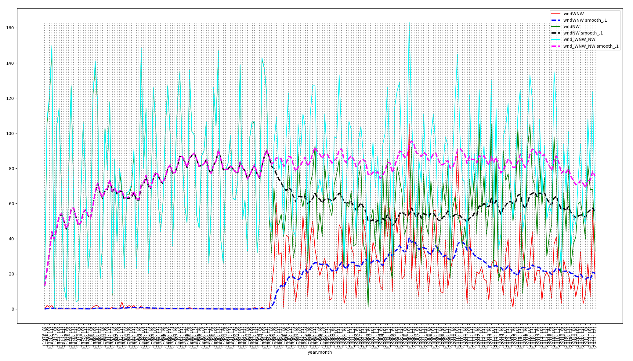
The dashed, exponential smoothing curves in the above graph compute a weighted estimate at each time step:
    Estimate_time = alpha X Value_time + (1 - alpha) X Estimate_time-1, with alpha = 0.1 in this plot.
The plot shows that adding WNW + NW restores the important NW level from 1995 onward.
Sometimes multi-year averaging can be useful to generate slopes across multiple years as an alternative to exponential smoothing.

1c. Remove all raptor attributes containing _All in their names except for your XX_All attributes.
    Keep XX_All, XX_All_log10, and XX_All_td for your XX in the data.
    Remove ONLY the other _All, _All_log10, and _All_td containing raptor attributes.

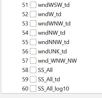
1d. Filter -> unsupervised -> attribute -> reorder the attributes to put your XX_All target attributes at the bottom of the 60.
    Here are my final 10 when XX is SS.
SS_All

1e. Save this file as XX_month_change.arff.gz, using the arff.gz format save, where XX is your raptor two-letter ID.
    You must turn this into D2L along with XX_week_change.arff.gz in a later step.

Q1: Remove your XX_All_td and XX_All_log10 temporarily and run the M5P regresssor. Record these results for XX_All as the target.
    (See the README.)

Q2: Temporarily remove year and month because they are not climate attributes, run M5P again, and record your results.
    (XX_All_td and XX_All_log10 are still out of the data. See the README.)

Q3: What climate attributes appear in the DECISION TREE part of Q2's answer. Do not look at the individual LM expressions.

Q4: Execute UNDO until restoring year, month, and all 3 XX_ attributes, or re-load your saved XX_month_change.arff.gz.
Remove your XX_All_td and XX_All temporarily and run the M5P regresssor, keeping XX_All_log10; year & month are in the data.
Record these results for XX_All_log10 as the target. (See the README.)

Q5: Temporarily remove year and month because they are not climate attributes, run M5P again, and record your results.
    (XX_All_td and XX_All are still out of the data. XX_All_log10 is the target. See the README.)

Q6: Compute the following ratios, where CC is correlation coefficient, our primary measure of model accuracy.
(CC of Q2) / (CC of Q1) shows drop in model correlation for XX_All after dropping time and using only climate.
    = N.n (the above ratio)
(CC of Q5) / (CC of Q4) shows drop in model correlation for XX_All_log10 after dropping time and using only climate.

Which target approach retains a higher percentage of CC-with-year-month after it has dropped year and month,
XX_All or XX_All_log10? Which gives better results overall in terms of CC, XX_All or XX_All_log10?

Q7: Run SimpleLinearRegression 5 times on the XX_All_log10 data, with XX_All, XX_All_td, year, and month OUT of the data.
After each run, record results in the README, then REMOVE the attribute selected by SimpleLinearRegression before making
the next test run. You are using the process of elimination for find the 5 most correlated climate attributes for SimpleLinearRegression
by finding, recording, and removing them, one at a time. See the README.

Q8: How do the 5 most important climate attributes selected by SimpleLinearRegression in Q7 compared with the 5 most important
in Q5? Answer is in term of attribute names, not numbers. See the README.

Q9: Restore the 5 attributes removed in Q7. We are still predicting XX_All_log10 with the following out of the data:
year, month, XX_All, and XX_All_td. Run the Select attributes Weka tab with default hyperparameters. Paste your results
per the README. How do the attributes selected by this step compare with those of Q5 and Q7 in terms of attribute names?

Q10. Turn XX_month_change.arff.gz into D2L.
*********************************************************
Q11 through Q20: Repeat steps Q1 through Q10 using the same XX as Q1 through Q10, but this time loading week_change.arff.gz,
analyzing its data, and saving XX_week_change.arff.gz.

One goal here is to determine whether higher resolution in terms of weekly time periods makes for more accurate or less accurate
CCs than monthly time periods, although there are no questions about that specfically. Just repeat Q1-Q10 using the weekly dataset.
The README Q11-Q20 contain the answer templates.

At the end you must turn in your completed README and files XX_month_change.arff.gz and XX_week_change.arff.gz by the due date.