CPSC 558 - Scripting for Data Science, Fall 2024,
Thursday 6:00-8:50 PM, Old Main 158 .
Assignment 2 is due via D2L Assignment 2 drop box by TBD.

Use Firefox or try other non-Chrome browser for these links. Chrome has problems.

Download & install Weka 3.8.6 (latest stable 3.8) from the website per our course page.

Then download handout files CSC223f24FRQDassn2.arff.gz and
README_558_Assn2.txt.
   
We are using data generated by an upcoming CPSC223 project, hence the file name.
You may need to control-click the README_558_Assn2.txt link in order to save it.
The former contains the starting data for this assignment and the latter has questions you must answer.
Place these files in a directory (folder) with the assignment name, e.g., CSC558Assn2.

You will turn in the following files via D2L Assignment 2 after completing the assignment per steps below.
README_558_Assn2.txt contains your answers. Make sure to use a text file format, not Word or other format.

When you have finished and checked your work:
Include these 3 files including README_558_Assn2.txt when you
turn in your assignment. If at all possible, please create them in a
single directory (folder) and turn in a standard .zip file of that
folder to D2L. I can deal with turning in all individual files, but
grading goes a lot faster if you turn in a .zip file of the folder.
You can leave CSC223f24FRQDassn2.arff.gz in there if you want.

    README_558_Assn2.txt
    CSC558Assn2Wavetype.arff.gz
    CSC558Assn2Dupl.arff.gz

This assignment builds on signal processing analysis begun in CSC558
back in spring 2020 and brought to its most recent state of straightforward prediction in CSC458 in spring 2024,

The modified dataset used in the current assignment adds significant, non-white-noise ambiguity to the prior
data by adding together multiple copies of a given waveform type with differing frequencies and amplitudes. You
must analyze this more complicated dataset, both for classification and regression. Please take notes
when I go over the predecessor data in class.

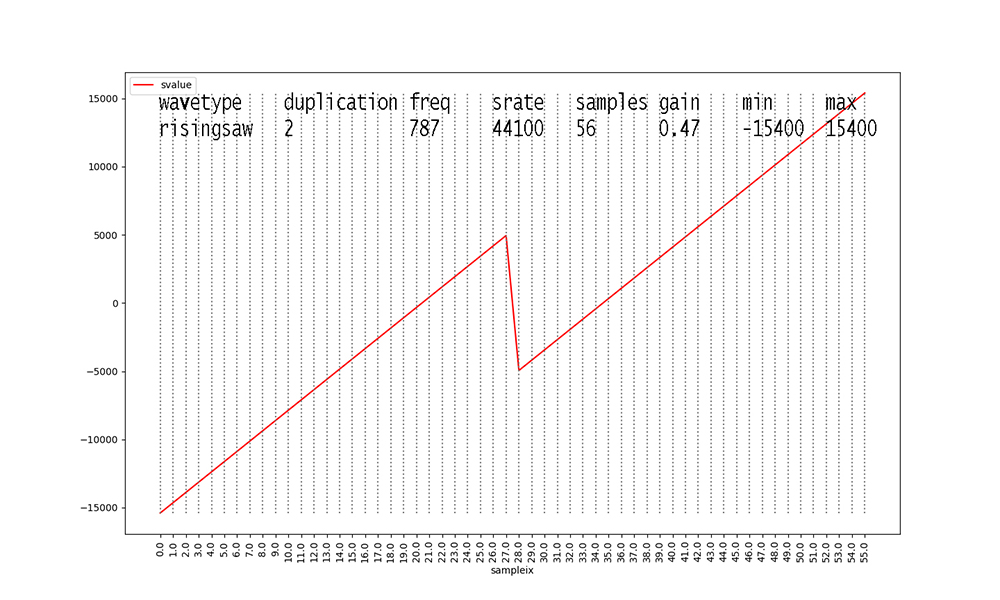
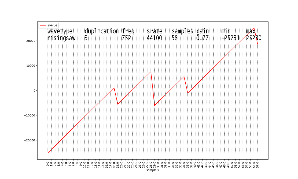
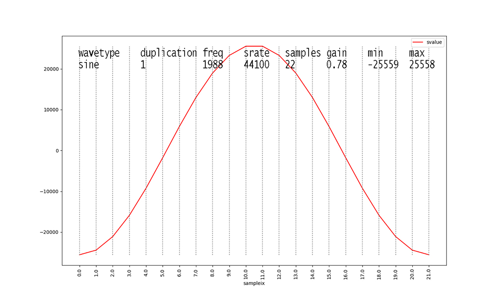
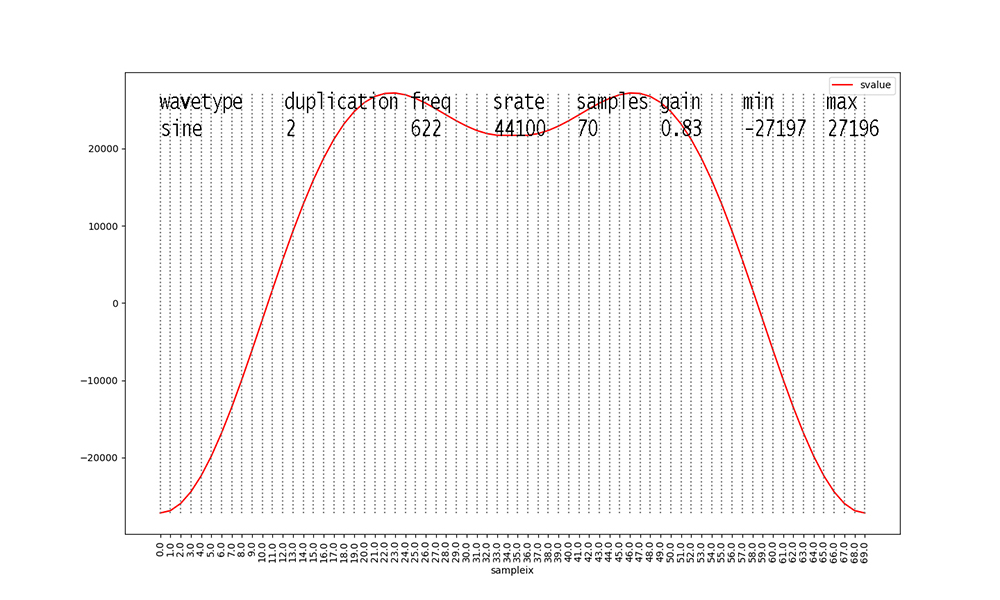
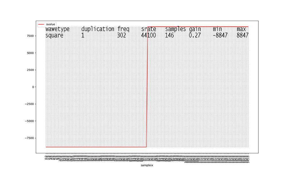
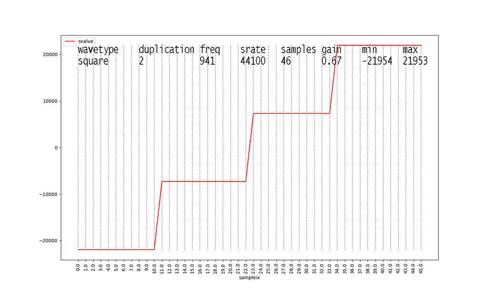
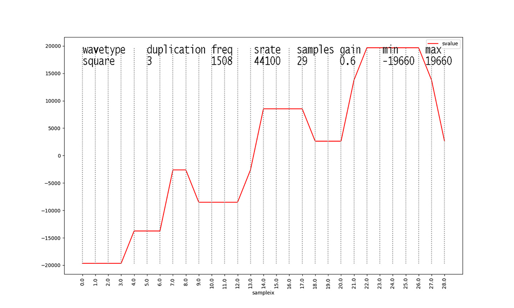
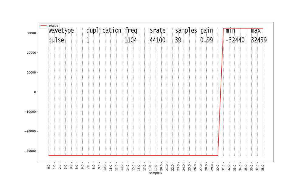
Examine Figures 1 through 18 as follows. First, look at the waveforms
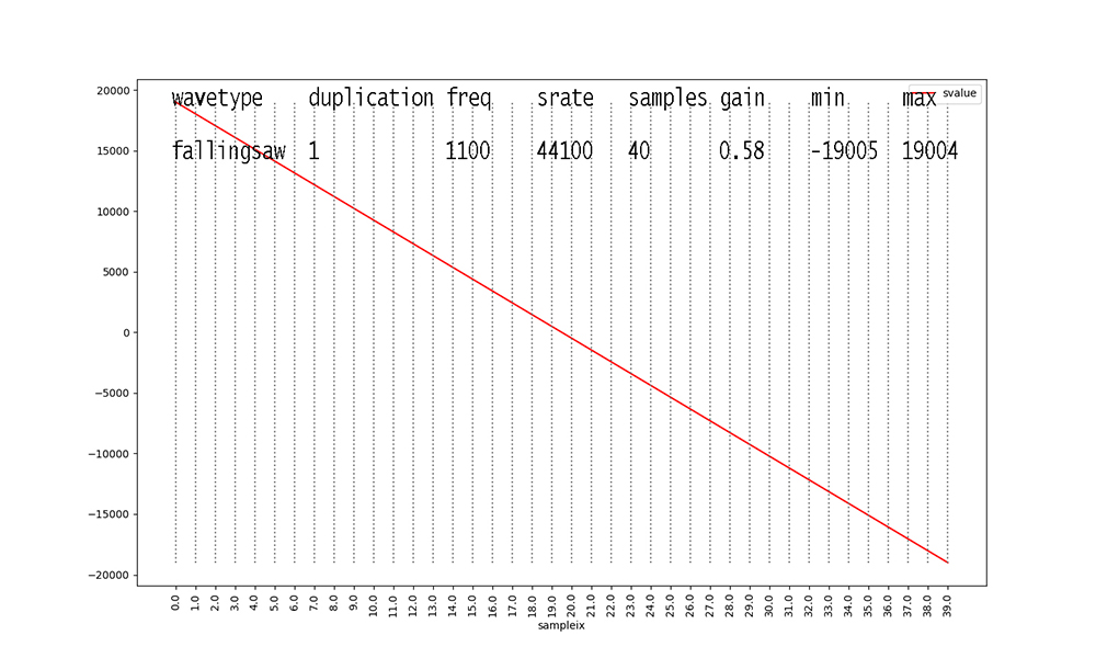
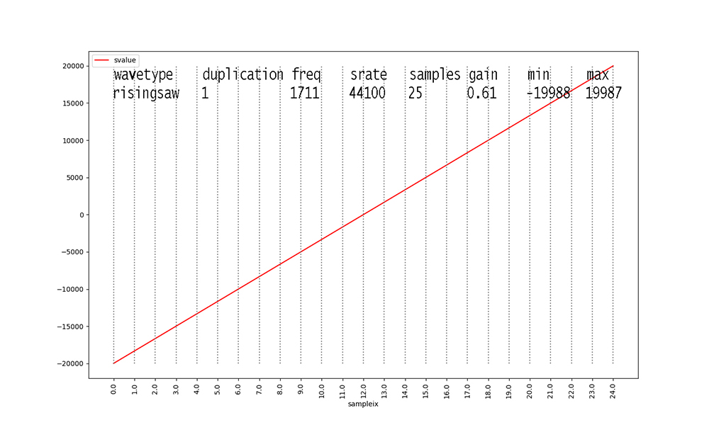
with duplication == 1 (Figures 1, 4, 7, 10, 13, 16).

These 6 waveforms are our primary waveforms. Our waveform generator from
CPSC223 generates 1 second's worth of digital audio samples at a standard sampling rate of
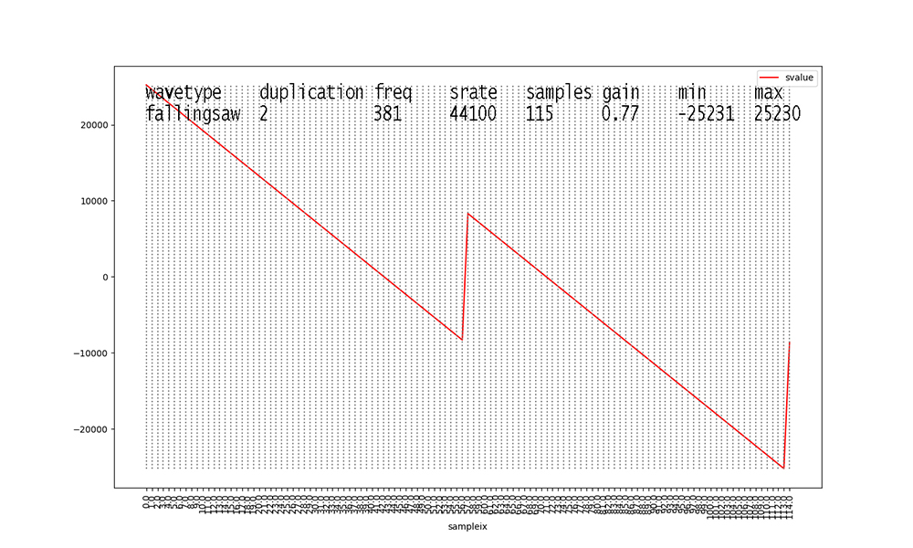
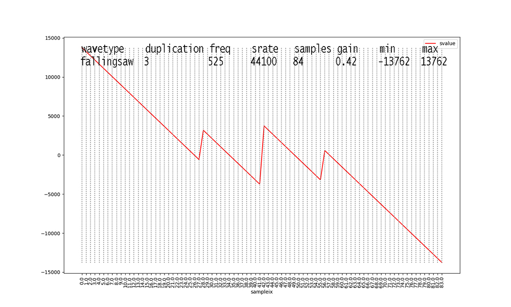
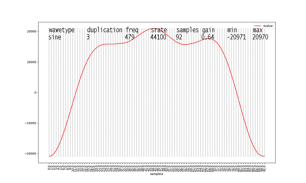
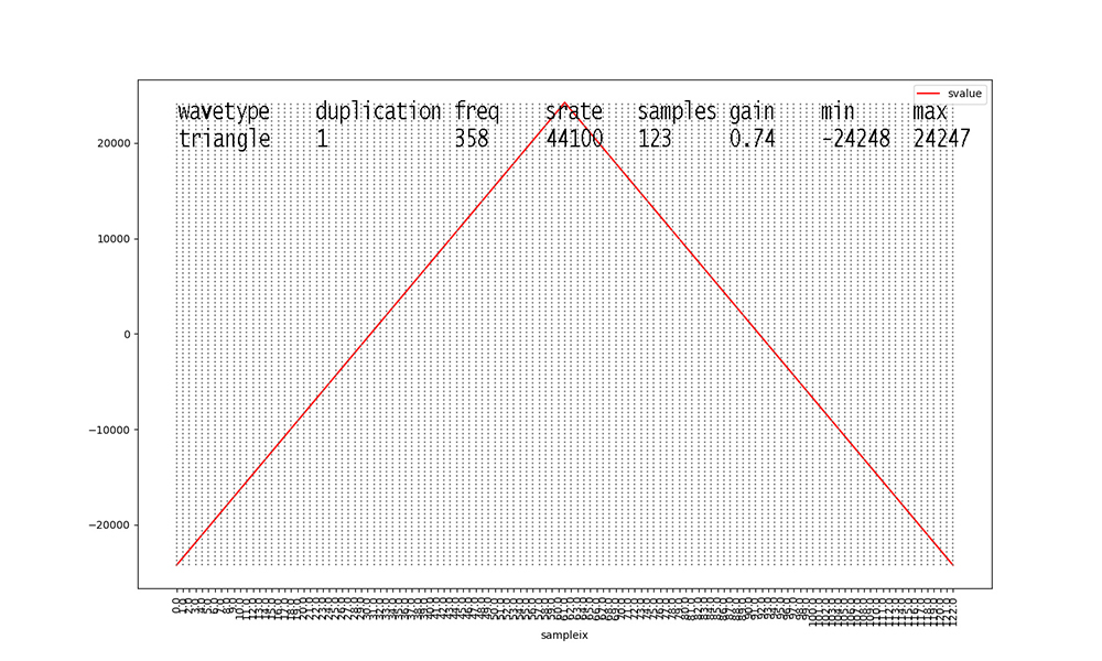
44,100 samples per second. Figures 1 through 18 show only 1 cycle of each waveform.
From the Python generator code,
    samples = math.floor(srate / freq), so with a constant srate of 44100,
Figure 1 shows 40 samples for a fundamental frequency of 1100 Hertz (cycles per second).
Higher frequencies yield fewer samples per waveform cycle in the data, and lower
frequencies yield more samples per waveform, as illustrated in Figures 1 through 18.

Signal amplitudes vary in the 16-bit integer range [-32768, 32767] per digital audio level standards.
The gain for a signal in our dataset scales this outer range down.
For example, 0.58 X 32767 = 19004 when rounded for Figure 1.

Figure 1

Figure 2

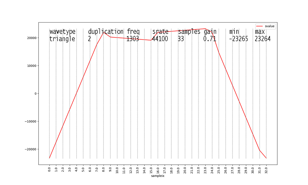
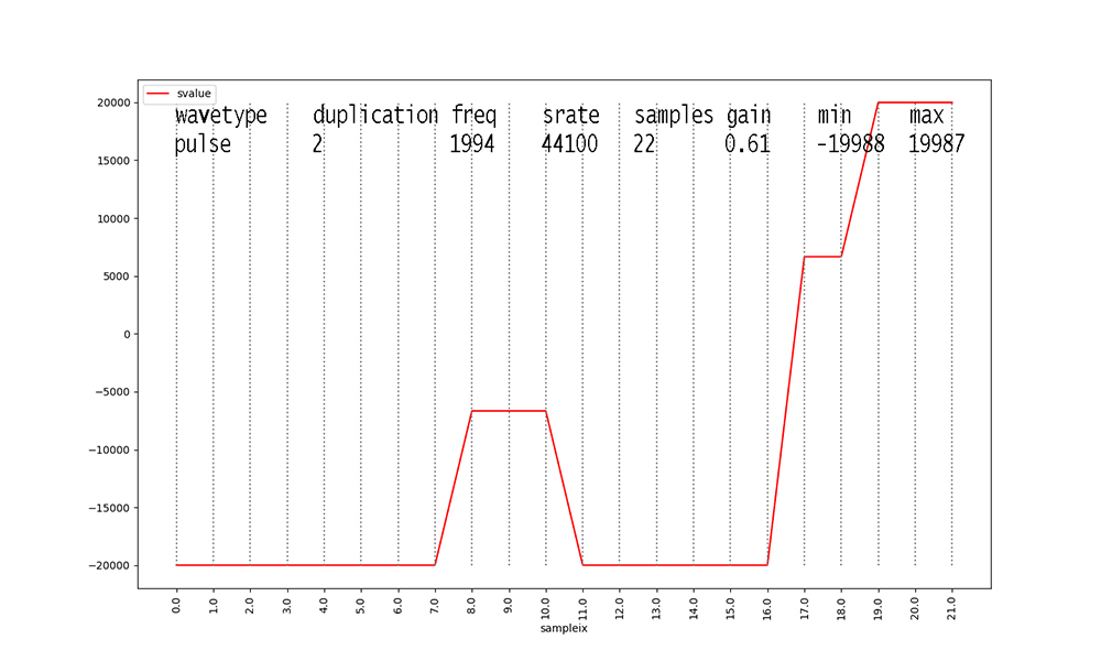
Figures with duplication values of 2 or 3 are new to this dataset this semester.
I added them to inject some ambiguity into the data.
Waveforms with duplication == 2 start to make these figures and their data analyses messy.

The original waveform with duplication == 1 is scaled down in amplitude X 0.666 and a
second identical waveform at 2 X the frequency and 0.333 the amplitude is added to its
samples before scaling the aggregate waveform by the stated gain.

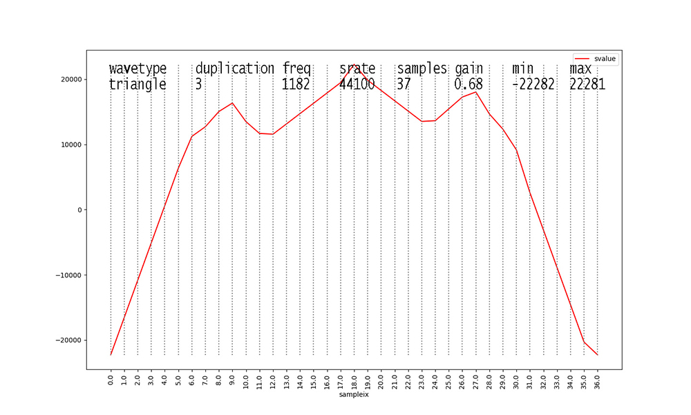
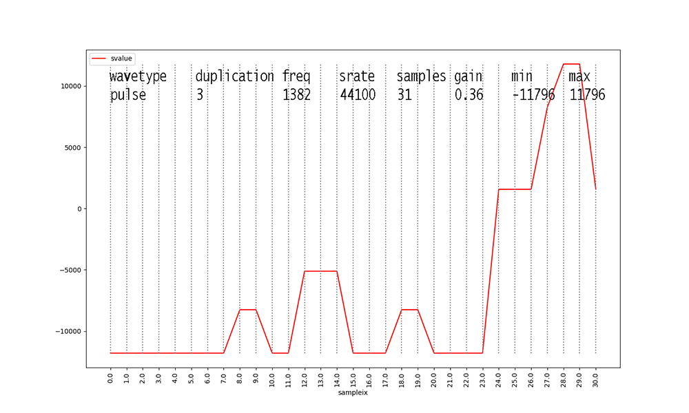
Finally, waveforms with duplication == 3 take the result of aggregate duplication == 2
waveforms and add another identical waveform at 3 X the original frequency and
0.15 X the amplitude, after scaling the aggregate duplication == 2 waveform samples
by 0.85 X their values. Scaling the aggregate waveform by the stated gain always occurs as the final step.
These steps in duplication occur to all of the waveform types with duplication values > 1.
Figure 3

Figure 4

Figure 5


Figure 6


Figure 7


Figure 8


Figure 9


Figure 10


Figure 11


Figure 12

Figure 13

Figure 14

Figure 15

Figure 16: Our pulse wave has a 20% duty cycle. The final 20% of a cycle's samples are high.

Figure 17

Figure 18

Here is a summary of the data attributes in CSC223f24FRQDassn2.arff.gz.

ampl1             The amplitude of the frequency-domain fundamental
                       frequency, normalized to the value 1.0 for all instances (rows of data).
freq1               The frequency of the frequency-domain fundamental
                       frequency, normalized to the value 1.0 for all instances (rows of data).
ampl2             The second-strongest amplitude (2nd harmonic) as a
                       fraction of ampl1.
freq2               The frequency of ampl2 as a multiple of ampl2.
ampl3, freq3 through ampl31, freq31 as stated above.
ampl32            The thirty-second-strongest amplitude (32nd harmonic) as a fraction of ampl1.
freq32              The frequency of ampl32 as a multiple of ampl32.
rawampl1          Is the actual non-normalized amplitude of the fundamental
                         frequency as extracted by the scipy FFT (Fast Fourier Transform) time-to-frequency domain library.
rawfreq1          Is the actual non-normalized frequency of the fundamental
                        as extracted by the FFT time-to-frequency domain library.

THE ABOVE ATTRIBUTES ARE FROM THE FREQUENCY DOMAIN EXTRACTION OF FFT.
THE FOLLOWING UP TO THE TAGGED ATTRIBUTES ARE FROM THE TIME DOMAIN,
WHICH HAS DISCRETE DIGITAL AUDIO SAMPLES 44100 TIMES PER SECOND.

P0                    is the leftmost sample value in this time-domain signal
reading left-to-right, small for rising waveforms, large for falling.
P25                  is the sample value 25% of the way across the
waveform going left-to-right.
P50                  is the sample value 50% of the way across the waveform going left-to-right.
P75 is the sample value 75% of the way across the waveform
going left-to-right.
P100                is the rightmost sample value in this signal reading left-to-right.
reversals           the number of times an increasing time-domain wave's
                         samples reverses to decreasing or vice versa, i.e.,
                         direction reversals.

MIN, MAX, MEAN, PSTDEV (population standard deviation) and MEDIAN (value in
the middle) are those statistical measures for one cycle of the waveform.
Unlike Assignment 1, P50 is not the same as MEDIAN. In the current assignment,
P50 is the signal sample 50% of the way across the waveform going left-to-right
in one waveform cycle, whereas MEDIAN looks at all individual discrete level
samples in one waveform and picks the one in the center of these sample values.

The followed 5 are TAGGED ATTRIBUTES, i.e., meta-data tagged onto this
dataset and not part of the actual waveform data. They are parameters to
the wave generators.

twavetype           one of {triangle,sine,square,pulse,risingsaw,fallingsaw}
tduplication        one of {1, 2, 3} as explained above for adding waves
tfreq               frequency of the fundamental sine wave component
tsrate              sampling rate, constarin of 44100 in this dataset
tgain               signal gain in the range [0.25, 1.0] as explained above

Inspect Weka's Preprocess tab showing histogram of Distribution values

STEP 1: Load CSC223f24FRQDassn2.arff.gz into Weka using the Preprocess ->
Open file... button.
    Set file type to arff.gz as in Assignment 1.

STEP 2: Remove all tagged attributes except twavetype, leaving 78 attributes.

All Qn questions must be answered in file README_558_Assn2.txt.