nCSC 458 - Data Mining & Predictive Analytics I, Spring 2024, Assignment 3 on Data Compression & Classification.

Assignment 3 due 11:59 PM Thursday March 21 via D2L Assignment 3.

The February 28 class will walk through this handout with any remaining time available for project work.

Q1 through Q11 in README.assn3.txt are worth 8% each and a correct CSC458assn3.arff.gz file is worth 12%. There is a 10% penalty for each day it is late to D2L.
 
1. To get the assignment:
Download compressed ARFF data file month_HM_reduced_aggregate.arff.gz and Q&A file README.assn3.txt from these links.
You must answer questions in README.assn3.txt and save & later turn in working file CSC458assn3.arff.gz.
Each answer for Q1 through Q11 in README.assn3.txt is worth 8 points, and
CSC458assn3.arff.gz with correct contents is worth 12%, totaling 100%. There is a 10% late penalty for each day the assignment is late, and it needs to be in before I go over my solution on March 27 to earn points.

2. Weka and README.assn3.txt operations
Start Weka, bring up the Explorer GUI, and open month_HM_reduced_aggregate.arff.gz.
    Set Files of Type at the bottom of the Open window to (*.arff.gz) to see the input ARFF file. Double click it.

This ARFF file has 45 attributes (columns) and 226 instances (rows) of monthly aggregate data from August through December of 1976 through 2021.
    Here are the attributes in the file. It is a monthly aggregate of daily aggregates of (mostly 1-hour) observation periods.

year                                                    1976-2021
month                                                  8-12
HMtempC_mean                                 mean for month of temp Celsius during observation times
WindSpd_mean                                  same for wind speed in km/hour
HMtempC_median                              median for month
WindSpd_median
HMtempC_pstdv                                population standard deviation
WindSpd_pstdv
HMtempC_min                                   minimum & maximum
WindSpd_min
HMtempC_max
WindSpd_max
wndN                                                 tally of North winds for all observations in the month, etc.
wndNNE
wndNE
wndENE
wndE
wndESE
wndSE
wndSSE
wndS
wndSSW
wndSW
wndWSW
wndW
wndWNW
wndNW
wndNNW
wndUNK
HMtempC_24_mean                    Changes in magnitude (absolute value of change) over 24, 48, and 72 hours
HMtempC_48_mean
HMtempC_72_mean
HMtempC_24_median
HMtempC_48_median
HMtempC_72_median
HMtempC_24_pstdv
HMtempC_48_pstdv
HMtempC_72_pstdv
HMtempC_24_min                    The min & max are their signed values.
HMtempC_48_min
HMtempC_72_min
HMtempC_24_max
HMtempC_48_max
HMtempC_72_max
SS_All                                        Tally of sharp-shinned hawk observations during each month 8-12, 1976-2021. Target attribute.

You can examine its contents and sort based on attributes by opening the file in the Preprocess Edit button.

2a. In the Preprocess tab open Filter -> unsupervised -> attribute -> AddExpression and add the following 4 derived attributes.

    Enter name SS_All_Range10 with an expression aN, where N is the attribute number of SS_All, which is our primary target attribute. (Use a45 for attribute 45, not "45" or "aN".) Apply.

        Be careful NOT TO INCLUDE SPACES within your derived attribute names.

    Enter name SS_All_EqFreq10 with an expression aN, where N is again the attribute number of SS_All. Apply.

    Enter name SS_All_Sqrt with an expression sqrt(aN), where N is the attribute number of SS_All. Apply.
        This step compresses the SS_All tally. (You can compare the min and the max of the original attribute
            in Weka's Preprocess upper-right panel against the sqrt by using a calculator. This approach also
            worls for log10 in the next step. Do NOT try it with the mean, which does not change linearly.)

    Enter name SS_All_Log10 with an expression log(aN+1)/log(10), where N is the attribute number of SS_All. Apply.
        This step compresses SS_All even more.
        The reason for adding +1 to aN is to avoid taking the log(0) for SS_All counts of 0, which is undefined. None will be negative.

    At this point you have 49 attributes.

2b. Select Filter -> unsupervised -> attribute -> Discretize to chop SS_All_Range10 and SS_All_EqFreq10 into 10 discrete classes as follows.

    Set the Discretize attributeIndices to the index of SS_All_Range10, leave the other Discretize parameters at their defaults (useEqualFrequency is False), and Apply.

    Set the Discretize attributeIndices to the index of SS_All_EqFreq10, set useEqualFrequency to True, leave the other Discretize parameters at their defaults, and Apply.

    Save this dataset as CSC458assn3.arff.gz, making sure "Files of Type" is set to (*.arff.gz) and the file is named correctly. It has 49 attributes.Turn in CSC458assn3.arff.gz when your turn in your README.assn3.txt to D2L.

Figures 1 through 5 show the statistical distributions of SS_All and these 4 derived attributes. Use the Preprocessor to make sure yours look the same.
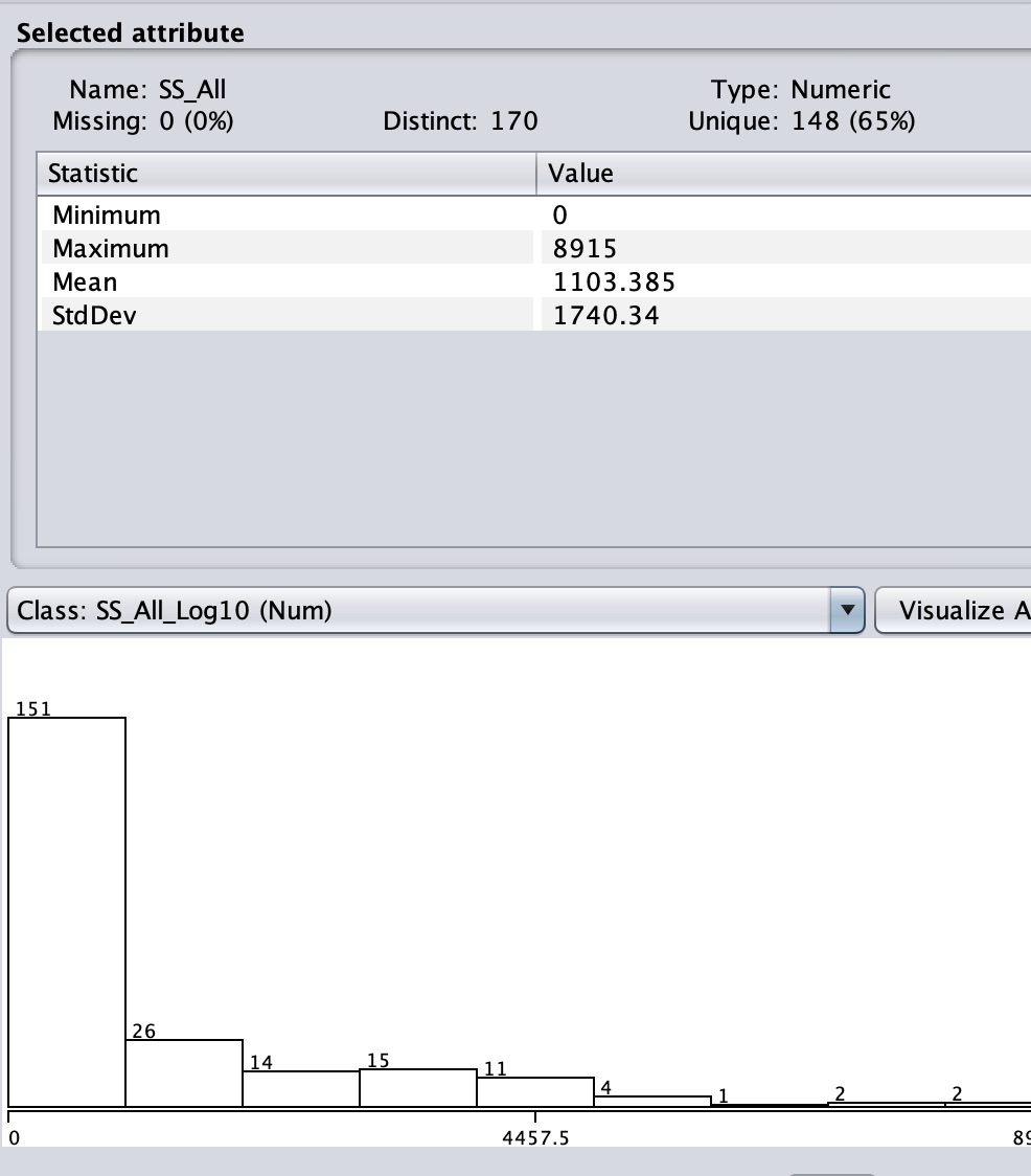
F1

Figure 1: SS_All

F2

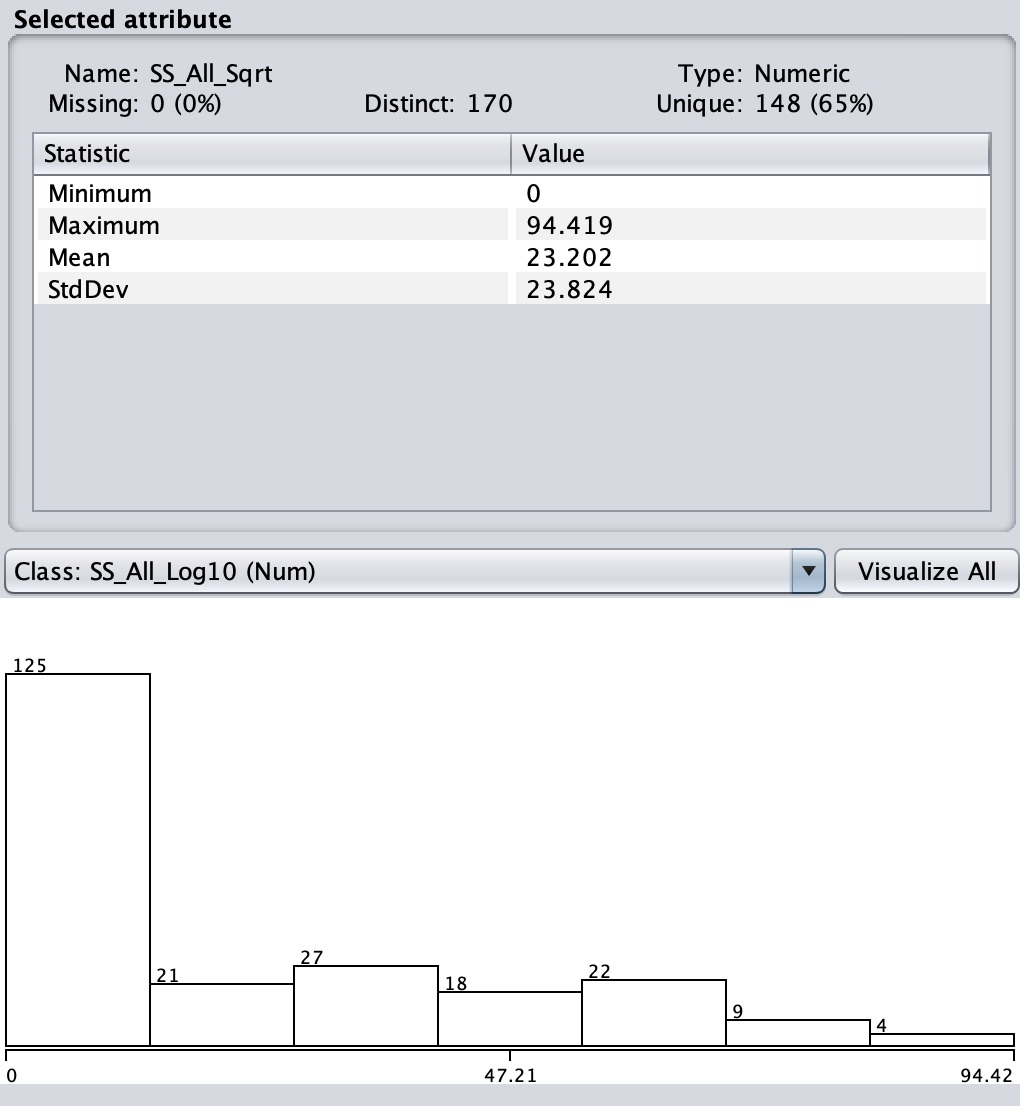
Figure 2: SS_All_Sqrt

F3

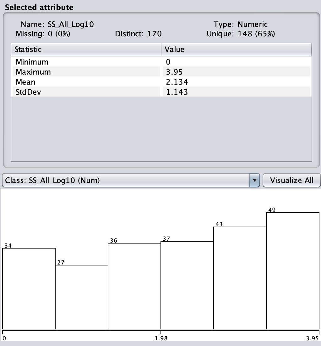
Figure 3: SS_All_Log10

F4

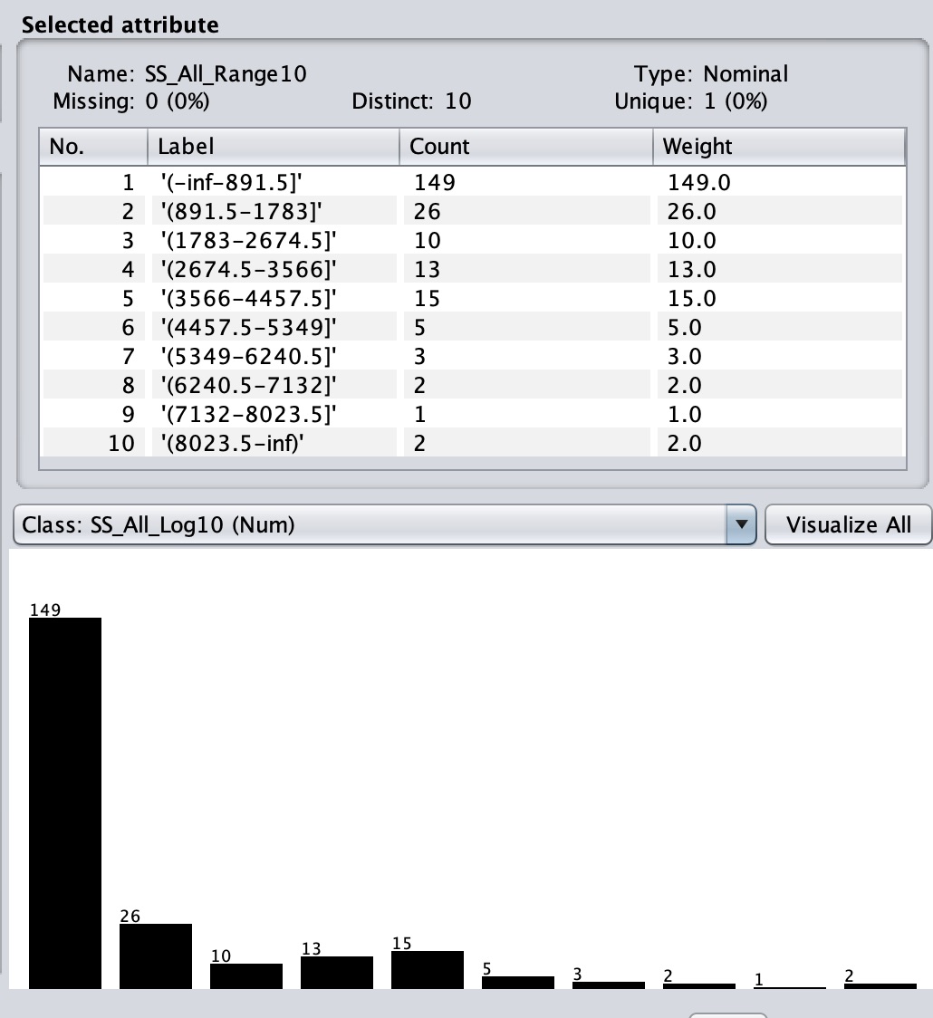
Figure 4: SS_All_Range10 (may be filled with white instead of black)

F5

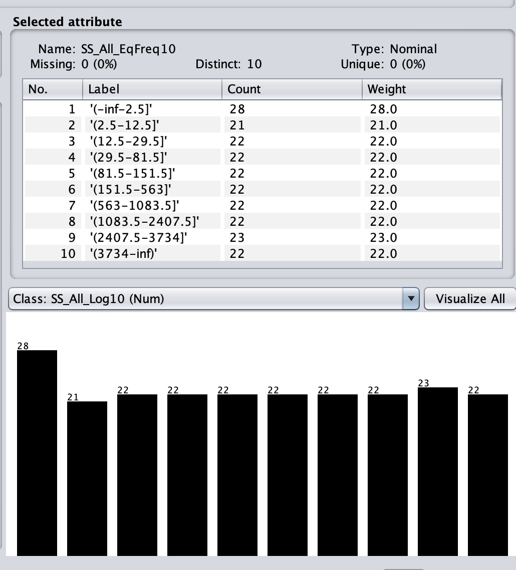
Figure 5: SS_All_EqFreq10

Check to sure that your distributions match Figures 1 through 5.

2c
. Remove derived attributes SS_All_Range10, SS_All_EqFreq10, SS_All_Sqrt, and SS_All_Log10 so that SS_All is the only target attribute, following non-target attribute HMtempC_72_max. We will use them later.

REGRESSION:

Q1: In the Classify TAB run rules -> ZeroR and fill in these numbers N.N below by sweeping the output with your mouse, hitting control-C to copy, and then pasting into README.assn3.txt, just like Assignment 2. What accounts for the predicted value of ZeroR? Examine the statistical properties of SS_All in the Preprocess tab to find the answer.

ZeroR predicts class value: N.N    (This is the predicted value of ZeroR.)
Correlation coefficient                 N.N  
Mean absolute error                   N.N
Root mean squared error               N.N
Relative absolute error                N      %
Root relative squared error            N      %
Total Number of Instances              226

Q2: In the Classify TAB run functions -> LinearRegression and fill in these numbers N.N below.

Correlation coefficient                 N.N  
Mean absolute error                   N.N
Root mean squared error               N.N
Relative absolute error                N      %
Root relative squared error            N      %
Total Number of Instances              226

Q3:
In the Classify TAB run trees -> M5P and fill in these numbers N.N below.

Correlation coefficient                 N.N  
Mean absolute error                   N.N
Root mean squared error               N.N
Relative absolute error                N      %
Root relative squared error            N      %
Total Number of Instances              226

Q4: In the M5P model tree of Q3, how many Rules (linear expressions) are there? Also, in the decision tree that precedes the first leaf linear expression "LM num: 1", what attributes are the key decision tree attributes in predicting SS_All? Copy & paste this section of the Weka output (the decision tree), and then list the attributes in the tree to ensure you see them all.

 M5 pruned model tree:
(using smoothed linear models)

Paste the decision tree that appears here in Weka's output.

LM num: 1


Q5: In the decision tree of Q4, the leaf nodes that point to linear expressions look like this:

|   |   |   |   ATTRIBUTE_NAME <= N.N : LM4 (13/26.17%)

In that leaf, 13 is the COUNT of the total 226 observation instances reaching that decision, 26.17% is an Error Measure (the root relative squared error just for that leaf, with 0.0% being the least and 100.0% being the worst error rate. LM4 in this example is the linear expression below the decision tree in Weka's output.

What month or months have the lowest
Error Measure (the root relative squared error) in Q4's decision tree? You can check the range of month values in Weka's Preprocess tab. Why do you think that is? Take a look at Figure 27 near the bottom of this section of the Hawk Mountain ongoing analysis.

https://acad.kutztown.edu/~parson/HawkMtnDaleParson2022/#SS


"
Figure 27 shows that the day-of-year of the first sighting (_1st in the legend), days of the 25%, 50%, and 75% of the sharp-shins (_25th, _50th, and _75th), and the days of the peak count (_peak) and final sighting (_last) have not changed incrementally since 1976."

Here is the day-of-year tables of when the months start from Python.
In [15]: from datetime import datetime                                         

In [16]: newyear = datetime(year=2021, month=1, day = 1)                                                                      
In [17]: for month in range(8,13):
    ...:     startmonth = datetime(year=2021, month=month, day=1)
    ...:     fromNY = startmonth - newyear
    ...:     print('month', month, 'starts at dayofyear', fromNY.days)                                                                      
month 8 starts at dayofyear 212
month 9 starts at dayofyear 243
month 10 starts at dayofyear 273
month 11 starts at dayofyear 304
month 12 starts at dayofyear 334
In [18]: fromNY = datetime(year=2021, month=12, day=31)-newyear                
In [19]: print('last day of 2021 is', fromNY.days+1)                           
last day of 2021 is 365

Why would the Error Measure be low during the month or months of the decision tree with the low error value?

Figure 6 below from Weka's Visualize tab showing monthly aggregate SS_All counts as a function of the month may help to figure out the answer.

F6

FIGURE 6: SS_ALL observations as a function of discrete month 8 through 12.

2d
. In Preprocess hit UNDO or re-load
CSC458assn3.arff.gz so you have all of the attributes derived from SS_ALL.

Remove derived attributes SS_All_Range10, SS_All_EqFreq10, SS_All_Sqrt, and SS_All so that
SS_All_Log10 is the only target attribute, following non-target attribute HMtempC_72_max.

Q6: In the Classify TAB run functions -> LinearRegression and fill in these numbers N.N  for
SS_All_Log10 prediction below.

Correlation coefficient                 N.N  
Mean absolute error                   N.N
Root mean squared error               N.N
Relative absolute error                N      %
Root relative squared error            N      %
Total Number of Instances              226


How does the LinearRegression Correlation coefficient for SS_All_Log10 in Q6 compare to the LinearRegression Correlation coefficient for SS_All in Q2? What might account for the change? Compare the monthly distribution and range of values in Figure 7 to Figure 6 in thinking about this.

F7


FIGURE 7: SS_ALL_Log10 observations as a function of discrete month 8 through 12.

Q7: In the Classify TAB run tree -> M5P and fill in these numbers N.N  for SS_All_Log10 prediction below. What change is there in M5P Correlation coefficient for SS_ALL_Log10 going from Q3 to Q7?

Correlation coefficient                 N.N  
Mean absolute error                   N.N
Root mean squared error               N.N
Relative absolute error                N      %
Root relative squared error            N      %
Total Number of Instances              226


Q8: Which regressor showed more substantial improvement in terms of Correlation coefficient and error measures, the changes in LinearRegression going from Q2 to Q6, or in M5P going from Q3 to Q7?

CLASSIFICATION

2e
. In Preprocess hit UNDO or re-load
CSC458assn3.arff.gz so you have all of the attributes derived from SS_ALL.

Remove derived attributes 
SS_All_Log10, SS_All_EqFreq10, SS_All_Sqrt, and SS_All so that SS_All_Range10  is the only target attribute, following non-target attribute HMtempC_72_max.

Q9: In the Classify TAB run rules -> OneR and fill in these numbers N.N  for SS_All_Range10 prediction below. Also paste OneR's RULE as outlined below. Also paste the Confusion matrix. Which non-target attribute does OneR use in predicting SS_All_Range10? How is its kappa accuracy measure, on the kappa scale of 0.0 to 1.0, as suggested by Landis & Koch on this page?

https://faculty.kutztown.edu/parson/fall2019/Fall2019Kappa.html


=== Classifier model (full training set) ===

The RULE to paste appears here.

Time taken to build model: ... seconds


Correctly Classified Instances         N               N.n %
Incorrectly Classified Instances        N               N.n %
Kappa statistic                          N.n
Mean absolute error                      N.n
Root mean squared error                  N.n
Relative absolute error                 N.n %
Root relative squared error             N.n %
Total Number of Instances              226


Q10: In the Classify TAB run trees -> J48 AFTER setting J48's configuration parameter minNumObj (click on J48 after selecting it to get the parameter popup) to 11, meaning 11 observations minimum per leaf node in the decision tree. I found 11 gives the best kappa result through trial and error. Fill in these numbers N.N  for SS_All_Range10 prediction below. Also paste J48's TREE. Numeric tags on leaf nodes like (29.0/9.0) give (Number Of Instances Reaching Here / Number of Those Incorrectly Classified). Also paste the Confusion matrix. How is this tree's kappa compared to OneR's in Q9 and in the Landis & Koch categories?


J48 pruned tree
------------------

THIS IS J48's tree position in Weka's output.

Number of Leaves  :     N

Correctly Classified Instances         N               N.n %
Incorrectly Classified Instances        N               N.n %
Kappa statistic                          N.n
Mean absolute error                      N.n
Root mean squared error                  N.n
Relative absolute error                 N.n %
Root relative squared error             N.n %
Total Number of Instances              226


2f. In Preprocess hit UNDO or re-load CSC458assn3.arff.gz so you have all of the attributes derived from SS_ALL.

Remove derived attributes 
SS_All_Range10, SS_All_Log10, , SS_All_Sqrt, and SS_All so that SS_All_EqFreq10 is the only target attribute, following non-target attribute HMtempC_72_max.

Q11: In the Classify TAB run rules -> OneR and fill in these numbers N.N  for SS_All_EqFreq10 prediction below. Also paste OneR's RULE as outlined below. Also paste the Confusion matrix. Which non-target attribute does OneR use in predicting SS_All_EqFreq10? How is its kappa accuracy measure, on the kappa scale of 0.0 to 1.0, as suggested by Landis & Koch on this page? How does the histogram-leveling effect per Figure 5 of SS_All_EqFreq10 in this question's kappa compare to the kappa of Q9 per Figure 4's SS_All_Range10 uncompressed values?

=== Classifier model (full training set) ===

The RULE to paste appears here.

Time taken to build model: ... seconds

Correctly Classified Instances         N               N.n %
Incorrectly Classified Instances        N               N.n %
Kappa statistic                          N.n
Mean absolute error                      N.n
Root mean squared error                  N.n
Relative absolute error                 N.n %
Root relative squared error             N.n %
Total Number of Instances              226


2g. Reread all questions and make sure you have answered all questions such as Landis & Koch categories for kappa and result-to-result comparisons.

Q1 through Q11 in README.assn3.txt are worth 8% each and a correct CSC458assn3.arff.gz file is worth 12%. There is a 10% penalty for each day it is late to D2L.