CPSC 558 - Scripting for Data Science, Fall 2024, Thursday 6:00-8:50 PM, Old Main 158
.
Assignment
1 is due via D2L Assignment 1 drop box
by 11:59 PM Saturday
September 21.
Use
Firefox or try other non-Chrome
browser for these links. Chrome
has problems
Download
& install Weka 3.8.6 (latest
stable 3.8) from the website per
our course page.
Then download handout files CSC558F24Assn1Handout.arff.gz
and README_558_Assn1.txt.
You may need to control-click README_558_Assn1.txt
in order to save it.
The former contains the starting data
for this assignment and the latter has
questions you must answer.
Place these files in a directory
(folder) with the assignment name, e.g.,
CSC558Assn1.
You will turn in the following files via
D2L Assignment 1 after completing the
assignment per steps below.
README_558_Assn1.txt contains your
answers. Make sure to use a text file
format, not Word or other format.
When you have finished and checked
your work:
Include these 7 files along with README_558_Assn1.txt
when you
turn in your assignment. If at all
possible, please create them in a
single directory (folder) and turn in a
standard .zip file of that
folder to D2L. I can deal with turning
in all individual files, but
grading goes a lot faster if you turn in
a .zip file of the folder.
You can leave
CSC558F24Assn1Handout.arff.gz in there
if you want.
CSC558F24Assn1Student.arff.gz
CSC558F24Assn1MinAttrs.arff.gz
handouttest.arff.gz
handouttrain.arff.gz
randomtest.arff.gz
randomtrain.arff.gz
tinytrain.arff.gz
STEP 1: Load
CSC558F24Assn1Handout.arff.gz
into Weka using the Preprocess
-> Open file... button.
Set file type to
arff.gz per the screen shots below.
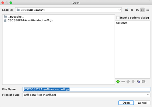
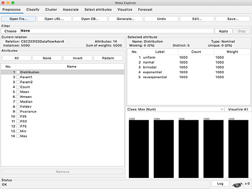
Figures 1 and
2: Loading the starting dataset into
Weka.
Assignment 1 analyzes statistical
measures extracted from 5
different generated
pseudo-random number distributions.
We will classify the name
of a record's distribution based on its
numeric statistical properties.
Later assignments will use real world
data. This assignment's data are
realistic for reasons that I explain
below.
Here are the 14 data attributes
(Excel or Weka columns) as enumerated
in Figure 2.
1. Distribution is one of uniform,
normal,
bimodal, exponential,
and revexponential as detailed
below.
My Python generating
script derives bimodal from normal
and derives revexponential from
exponential.
2 & 3. Param1 and Param2
are parameters to statistical generators
for the distributions. They differ by
generator.
4. Count is the number of numeric
distributions for each record (row) from
which my script has extracted stats.
5. Mean is the average value
within that record's distributions,
i.e., sumOfValues / Count.
6. Hmean is the harmonic mean,
which is the reciprocal of the (mean of
the reciprocals of the numbers),
sometimes used when
averaging ratios.
7. Median is the statistical
"value in the middle" of that record's
distributions, the mean of the two
middle values for even counts.
8. Pstdev is the population
standard deviation, a measure of
variability.
9. Pvariance is the square of the
Pstdev.
10-12. P25, P50, and P75
are the 25th, 50th,
and 75th percentiles, i.e.,
value at which 25%, 50%, and 75% of
a record's
distributions of values reading from
left (min value) to right (max value).
13 & 14. Min and Max
are the minimum and maximum of a
record's distributions of values.
The Python
script that generated this data is
here.
All of this assignment's numeric
distributions are normalized
into the range [1, 100] by my code.
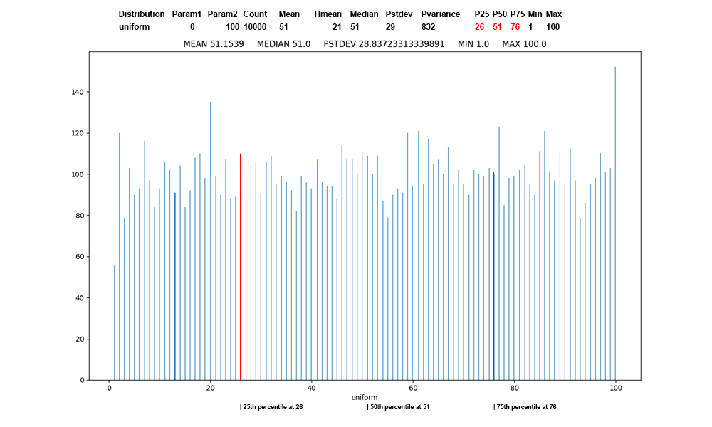
Figure 3: Uniform
distribution of 10,000 values, first
record of uniform data, red at the
percentile boundaries.
This is the classic "random
distribution". Random surveillance
(non-volunteer) testing during COVID
restrictions
to get an unbiased sample would be one
example. Rolling dice or shuffling cards
try for uniform distributions.
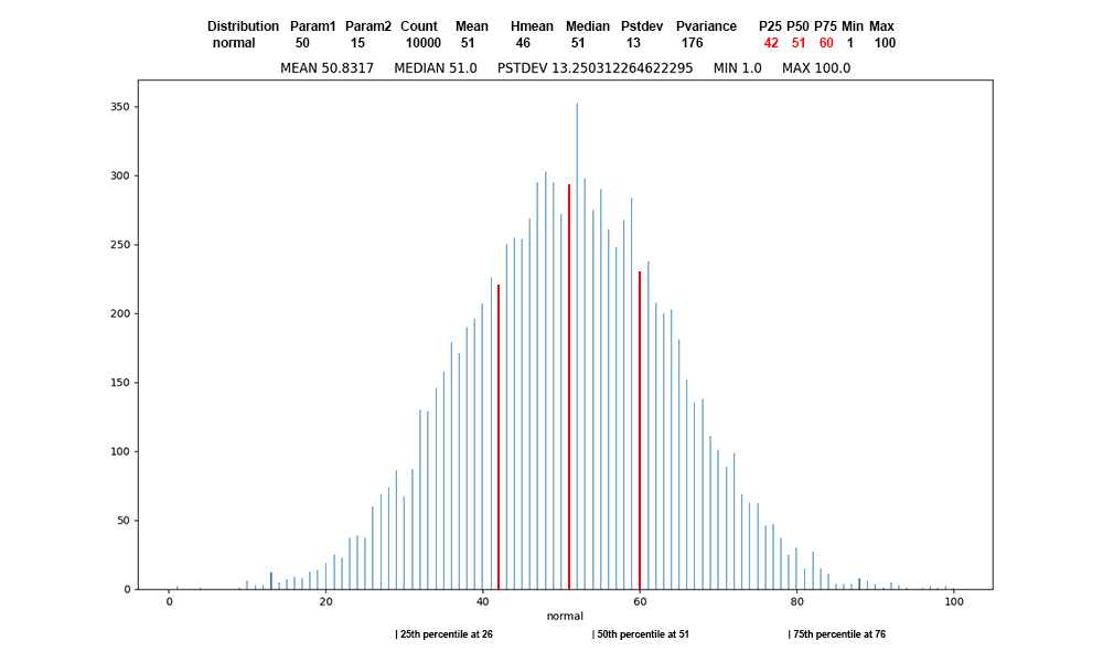
Figure
4: Normal
distribution
of 10,000
values, first
record of normal
data, red
at the
percentile
boundaries.
There
are many
manifestations
of the normal
distribution.
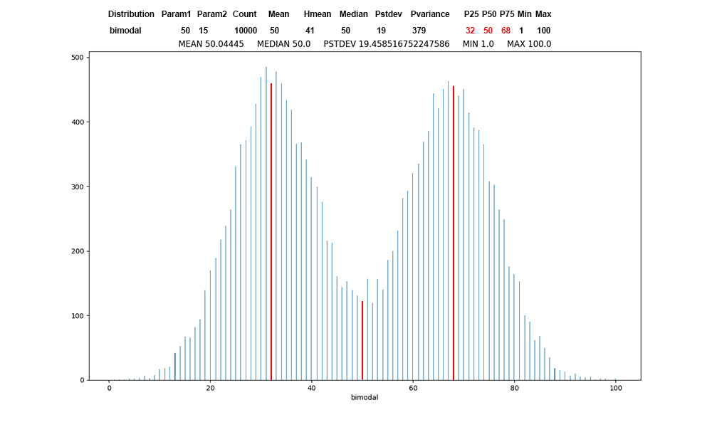
Figure
5: Bimodal
distribution
of 10,000
values, first
record of bimodal
data, red
at the
percentile
boundaries.
Bimodal
distribution
represents two
population
centers.
Occasionally
this appears
in project
grades.
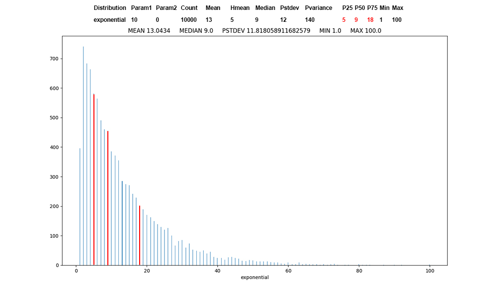
Figure 6: Exponential
distribution of 10,000 values, first
record of exponential data, red at the
percentile boundaries.
Unprotected COVID infection
propagates at an exponential
rate. For the alpha infection rate
of 3.5,
each unprotected
person infects 3 other unprotected
persons with a 100% probability, with a
50% probability of infecting a fourth.
I
have used exponential in teaching
Operating Systems to model
IO-bound threads, where most CPU bursts
are small.
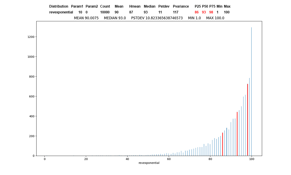
Figure 7: Revexponential
distribution of 10,000 values, first
record of revexponential data,
red at
the percentile boundaries.
Reverse exponential is just the
mirror image of exponential.
I
have used it
in teaching
Operating
Systems to
model
CPU-bound
threads, where
most CPU
bursts are
large.
STEP
2: Run filter
->
unsupervised
->
attribute
-> Reorder,
moving
attribute Distribution
to the last
position 14
while
maintaining
the relative
order of the
remaining 13
attributes. We
are doing this
because Weka
expects the class
attribute,
a.k.a. target
attribute,
to be the
final
attribute in
the data.
Always Apply
Weka's filters
one time
and inspect
the Preprocess
panels to
ensure your
work has taken
effect.
STEP 3: After
reviewing the 14 attributes in Weka's
Preprocess tab, run filter ->
unsupervised -> attribute ->
RemoveUseless. There should now be
11 attributes.
All Qn questions require answers
in README_558_Assn1.txt.
Each of Q1 through Q15 is worth 6.66% of
the assignment.
Please answer all questions, even if you
need to guess one.
It creates the opportunity for partial
credit. A lack
of an answer = 0% for that one. Also,
the penalty for missing
or incorrect files for Q15 is scaled by
severity.
Q1: Which attributes did RemoveUseless
remove? Why did it remove them?
(Help: You can click any Weka command
line and click More to read its
documentation.)
STEP 4:
Manually Remove attributes Param1
and Param2, leaving 9 attributes
intact.
We are removing them because they are tagged
attributes, a.k.a. meta-data,
that helps
to configure the Distribution
generators. Their values correlate
trivially with Distribution
since they helped to generate its
values. We are using only statistical
numeric data to
predict the associated Distribution,
also a tagged attribute.
STEP 5: Save this 9-attribute,
5000-instance dataset as CSC558F24Assn1Student.arff.gz
using the arff.gz output file format
shown in Figure 8. You will turn this
file in along with
several other files when you have
completed your work.
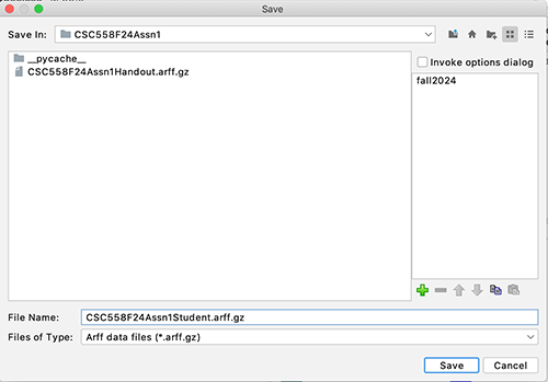
Figure 8:
Saving CSC558F24Assn1Student.arff.gz
as an arff.gz
file
Q2: In Weka's Classify tab run
classifier rules -> ZeroR and
paste ONLY these output fields
into your README file, substituting
actual values for the N and N.n
placeholders.
You must use control-C to copy Weka
output after sweeping the output to
copy.
Correctly Classified
Instances
N
N %
Incorrectly Classified
Instances
N
N %
Kappa
statistic
N
Mean absolute
error
N.n
Root mean squared
error
N.n
Relative absolute
error
N %
Root relative squared
error
N %
Total Number of
Instances
5000
=== Confusion Matrix ===
a
b c
d e <--
classified as
N
N N
N N | a =
uniform
N
N N
N N | b =
normal
N
N N
N N | c =
bimodal
N
N N
N N | d =
exponential
N
N N
N N | e =
revexponential
Q3: What are the "Correctly
Classified
Instances"
as a percentage and the Kappa value?
What accounts for this Kappa value in
terms of how ZeroR works for
classification?
(Help: Clicking "More" on the ZeroR
command line may help.)
Q4: In Weka's Classify tab run
classifier rules -> OneR and
paste ONLY
these output fields into your README
file, substituting actual values
for the N and N.n placeholders. In what
"Landis
and Koch" category
does this Kappa value fit?
Landis
and Koch
category:
Attribute
name:
<
N.n
->
exponential
<
N.n
-> normal
<
N.n
-> bimodal
<
N.n
-> uniform
>=
N.n
->
revexponential
(N/N instances
correct)
Correctly
Classified
Instances
N
N
%
Incorrectly
Classified
Instances
N
N
%
Kappa
statistic
N
Mean
absolute
error
N.n
Root
mean squared
error
N.n
Relative
absolute
error
N
%
Root
relative
squared
error
N
%
Total
Number of
Instances
5000
===
Confusion
Matrix ===
a
b
c
d
e
<--
classified as
N
N
N
N
N
|
a = uniform
N
N
N
N
N
|
b = normal
N
N
N
N
N
|
c = bimodal
N
N
N
N
N
|
d =
exponential
N
N
N
N
N
|
e =
revexponential
Q5:
In Weka's
Classify tab
run classifier
trees ->
J48 and
paste ONLY
these output
fields into
your README
file,
substituting
actual values
for the N and
N.n
placeholders.
In what "Landis
and Koch"
category
does this
Kappa value
fit?
Landis
and Koch
category:
J48 pruned
tree
------------------
AttrName <=
N
|
AttrName <=
N: exponential
(N.n)
|
AttrName >
N
|
|
AttrName <=
N: normal
(N.n)
|
|
AttrName >
N:
revexponential
(N.n)
AttrName >
N
|
AttrName <=
N: bimodal
(N.n)
|
AttrName >
N: uniform
(N.n)
Number of
Leaves
:
N
Size of the
tree : N
Correctly
Classified
Instances
N
N
%
Incorrectly
Classified
Instances
N
N
%
Kappa
statistic
N
Mean
absolute
error
N.n
Root
mean squared
error
N.n
Relative
absolute
error
N
%
Root
relative
squared
error
N
%
Total
Number of
Instances
5000
===
Confusion
Matrix ===
a
b
c
d
e
<--
classified as
N
N
N
N
N
|
a = uniform
N
N
N
N
N
|
b = normal
N
N
N
N
N
|
c = bimodal
N
N
N
N
N
|
d =
exponential
N
N
N
N
N
|
e =
revexponential
STEP 6: Note
the attributes used in the OneR rule of
Q4 and the J48 decision tree of Q5.
Remove ALL other attributes except for
these noted ones plus target attribute
Distribution,
which you must also keep. There should
be 4 attributes including Distribution.
Save this file
as CSC558F24Assn1MinAttrs.arff.gz
using the arff.gz format as before.
Q6:
In Weka's
Classify tab
run classifier
trees ->
J48 on
this MinAttrs
dataset
and paste ONLY
these output
fields into
your README
file,
substituting
actual values
for the N and
N.n
placeholders.
In what "Landis
and Koch"
category
does this
Kappa value
fit?
Landis
and Koch
category:
J48 pruned
tree
------------------
AttrName <=
N
|
AttrName <=
N: exponential
(N.n)
|
AttrName >
N
|
|
AttrName <=
N: normal
(N.n)
|
|
AttrName >
N:
revexponential
(N.n)
AttrName >
N
|
AttrName <=
N: bimodal
(N.n)
|
AttrName >
N: uniform
(N.n)
Number of
Leaves
:
N
Size of the
tree : N
Correctly
Classified
Instances
N
N
%
Incorrectly
Classified
Instances
N
N
%
Kappa
statistic
N
Mean
absolute
error
N.n
Root
mean squared
error
N.n
Relative
absolute
error
N
%
Root
relative
squared
error
N
%
Total
Number of
Instances
5000
===
Confusion
Matrix ===
a
b
c
d
e
<--
classified as
N
N
N
N
N
|
a = uniform
N
N
N
N
N
|
b = normal
N
N
N
N
N
|
c = bimodal
N
N
N
N
N
|
d =
exponential
N
N
N
N
N
|
e =
revexponential
STEP 7: So
far we have been using 10-fold
cross-validation for testing, in which
90%
of the records randomly selected are
used for training, the remaining 10% for
testing,
repeated 10 times using different 10%
for testing each time. Now we are going
to create
distinct training and testing datasets.
In Weka Preprocess tab run filter unsupervised
->
instance -> RemovePercentage
with the default arguments of 50%. There
should be
2500 instances after Apply. Look
at the distribution of Distribution
values in the Preprocess
tab. Save this dataset as
handouttest.arff.gz using the arff.gz
format as before.
STEP 8: Load
CSC558F24Assn1MinAttrs.arff.gz
to get all 5000 instances back. In
Weka
Preprocess tab
click the
RemovePercentage
command line
and set the invertSelection
parameter to True.
Run filter unsupervised
->
instance ->
RemovePercentage. There should again be
2500 instances
after Apply.
Look at the
distribution
of
Distribution
values in the
Preprocess
tab. Save
this dataset
as
handouttrain.arff.gz
using the
arff.gz
format as
before.
STEP 9:
In the
Classify
tab select Supplied
test set
and set it to
handouttest.arff.gz
per
Figure 9.
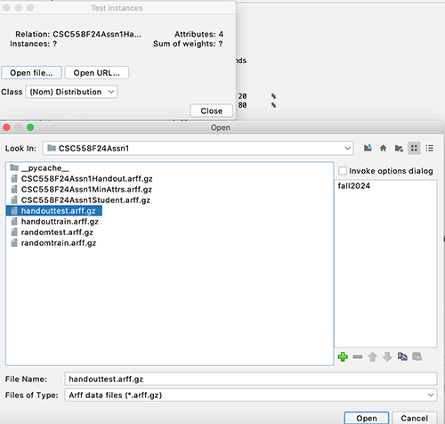
Figure 9:
Preparing to run distinct training
versus testing datasets.
Q7:
In Weka's
Classify tab
run classifier
trees ->
J48 on handouttest.arff.gz,
having trained
on handouttrain.arff.gz,
and
paste ONLY the
output fields
that
you pasted for
Q6 into
your README
file,
substituting
actual values
for the N and
N.n
placeholders.
In what "Landis
and Koch"
category
does this
Kappa value
fit? Consider
the
distribution
of
Distribution
values you
inspected
in STEPS 7 and
8 and the J48
decision tree
and the
Confusion
Matrix of Q7,
where only the
counts on the
diagonal represent
correctly
classified
target values.
Why did Q7
lead to the
Kappa value
you recorded
here in terms
of training
versus testing
data and
possible
over-fitting
of the J48
model to the
training data?
Each
column gives a prediction.
a
b
c
d
e
<--
classified
as Each
row is the
actual class
value.
N
N
N
N
N
|
a = uniform
N
N
N
N
N
|
b = normal
N
N
N
N
N
|
c = bimodal
N
N
N
N
N
|
d =
exponential
N
N
N
N
N
|
e =
revexponential
STEP
10: Load CSC558F24Assn1MinAttrs.arff.gz
to get all
5000 instances
back. In
Weka
Preprocess tab
click filter unsupervised
->
instance ->
Randomize
and hit Apply
ONE
TIME
with the
default
parameters.
Randomize
shuffles the
order of the
instances.
Now run RemovePercentage
with the invertSelection
parameter
set to the
default False.
There
should
be 2500
instances
after Apply.
Look at the
distribution
of
Distribution
values in the
Preprocess
tab. Save
this dataset
as
randomtest.arff.gz
using the
arff.gz
format as
before.
Then Undo
ONE
TIME
(careful not
to Undo the
Randomize!),
verify that
there are 5000
instances, run
RemovePercentage
after
setting the
invertSelection
parameter set
to True. Apply
should
again give
2500
instances.
Look
at the
distribution
of
Distribution
values in the
Preprocess
tab.
Save
this dataset
as
randomtrain.arff.gz
using the
arff.gz
format.
STEP
11: In the
Classify
tab select Supplied
test set
and set it to
randomtest.arff.gz
similar to
Figure 9.
Q8: In
Weka's
Classify tab
run classifier
trees ->
J48 on randomtest.arff.gz,
having trained
on randomtrain.arff.gz,
and paste ONLY
the output
fields that
you pasted for
Q6 and
Q7 into
your README
file,
substituting
actual values
for the N and
N.n
placeholders.
In what "Landis
and Koch"
category does
this
Kappa value
fit? Consider
the
distribution
of
Distribution
values you
inspected
in STEP 10 and
the J48
decision tree
and the
Confusion
Matrix of Q8,
where only the
counts
on the
diagonal
represent
correctly
classified
target values.
Why did Q8
lead to the
Kappa value
you recorded
here in terms
of training
versus testing
data as
compared with
the Kappa
value of Q7?
STEP 12:
Load randomtrain.arff.gz
into Weka in the Preprocess tab, run RemovePercentage
with the
invertSelection
parameter set
to False
and the percentage
set to 99.0
and Apply
ONE
TIME.
There
should be only
25 training
instances
remaining.
Again,
run
RemovePercentage
with the
invertSelection
parameter set
to False
and the percentage
set to 40.0
and Apply
ONE
TIME.
There
should be only
15 training
instances
remaining.
Look
at the
distribution
of
Distribution
values in the
Preprocess
tab. Save
this dataset
as
tinytrain.arff.gz
using the
arff.gz
format as
before.
STEP
13: In the
Classify
tab select Supplied
test set
and set it to
randomtest.arff.gz
similar to
Figure 9.
Q9:
In Weka's
Classify tab
run classifier
trees ->
J48 on randomtest.arff.gz,
having trained
on tinytrain.arff.gz,
and paste ONLY
the output
fields that
you pasted for
Q6 and
Q7 and
Q8 into
your README
file,
substituting
actual values
for the N and
N.n
placeholders.
In what "Landis
and Koch"
category does
this
Kappa value
fit? Consider
the
distribution
of
Distribution
values you
inspected
in STEP 13 and
the J48
decision tree
and the
Confusion
Matrix of Q9,
where only the
counts
on the
diagonal
represent
correctly
classified
target values.
Why do you
think Q9
leads to the
Kappa value
you recorded
here in terms
of training
versus testing
data as
compared with
the Kappa
value of Q8?
Q10:
In Weka's
Classify tab
run
instance-based
classifier lazy
-> IBk on
randomtest.arff.gz,
having trained
on tinytrain.arff.gz,
and paste ONLY
the output
fields that
you pasted for
Q9 (there
is no tree)
into your
README file,
substituting
actual values
for the N and
N.n
placeholders.
In what "Landis
and Koch"
category does
this
Kappa value
fit? Why do
you think Q10
leads to the
Kappa value
you recorded
here in terms
of training
versus testing
data as
compared with
the Kappa
value of Q9?
Q11: In
Weka's
Classify tab
run
instance-based
classifier lazy
-> KStar
on
randomtest.arff.gz,
having trained
on tinytrain.arff.gz,
and paste ONLY
the
output fields
that you
pasted for Q10
(there is no
tree) into
your README
file,
substituting
actual values
for the N and
N.n
placeholders.
Where IBk of
Q10
uses
K-nearest-neighbors
(KNN) linear
distance
comparisons
between each
test instance
and individual
training
instances (K=1
nearest
neighbor
by default),
KStar uses a
non-linear,
entropy
(distinguishability)
distance
metric. In
what "Landis
and Koch"
category does
this Kappa
value fit?
Inspect
misclassified
instance
counts in the
Confusion
Matrix, i.e.,
the
ones that are
NOT on the
diagonal. For
each
misclassified
count,
complete
the table
showing
PREDICTED
(column),
ACTUAL (row),
and the
misclassified
COUNT.
PREDICTED
(column)
ACTUAL
(row)
COUNT
STEP
14: Load CSC558F24Assn1MinAttrs.arff.gz
into Weka. The
remaining
interpretive
questions
relate to the
relationship
of the 3
non-target
attributes to
class
Distribution
and the graphs
of Figures 3
through 7.
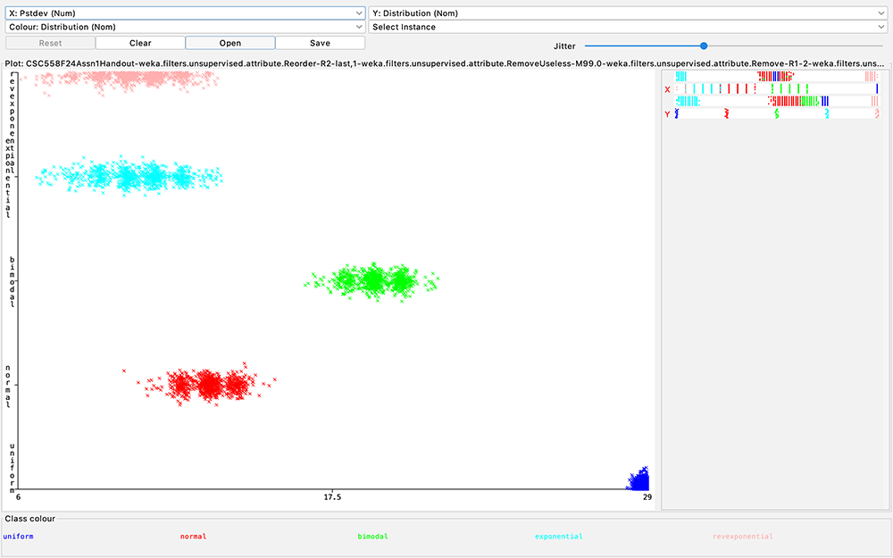
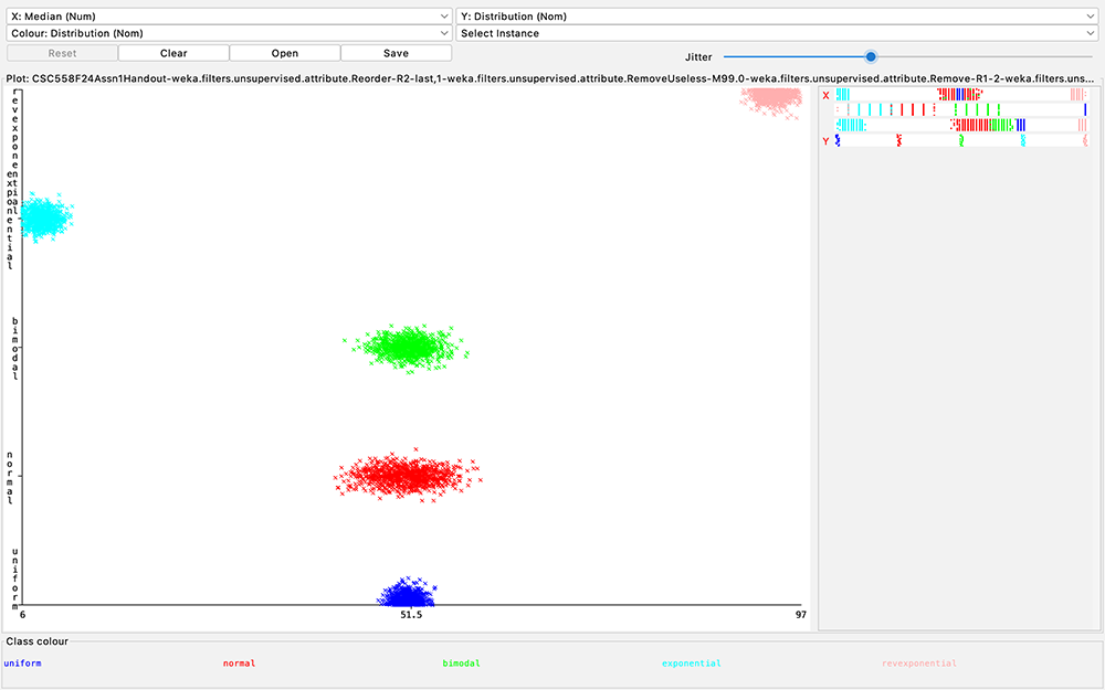
Figure
10: Scatter
plot of
Distribution
class (Y axis)
as a function
of Pstdev (X
axis)
Q12:
Inspect the
J48 decision
tree of your
answer for Q5,
Q6, or Q8.
(The trees
should be
identical).
Look at Figure
10 in the
handout.
What values of
target
attribute
Distribution
are
unambiguously
correlated
with Pstdev
without
referring to
any other
non-target
attributes?