CSC 523 - Advanced DataMine for Scientific Data Science, Fall 2023, M 6-8:45 PM, Old Main 158.

Assignment 4 Specification, code & README.txt are due by end of Friday December 8 via make turnitin on acad or mcgonagall.

DUE DATE MOVED TO END OF SUNDAY DEC 10 due to a glitch in access to student file system.
Even if you cannot see your files on acad, a student has informed me that ssh'ing into mcgonagall works OK.

     Do not round the return result from calling mean(history) in makeAveragingClosure(Nyears, attributeColumnNumber)'s
        nested closure function averager(row). The comments are correct with no rounding, which will give a diff.
        Here is what my code does: return mean(history)

11/27 Clarification regarding line 458 in handout file :
457 #   Dr. Parson is supplying the code for '_sm6' and '_sm4' STEP 4.
458     for CSVfileName in CSV2data.keys():
459         for trender, dataIndex in (('_sm6', 6), ('_sm4', 8)):
If you do a copy, paste, & edit of my STUDENT 4 portion, just use the loop starting at line 459 above.
Do not copy "for CSVfileName in CSV2data.keys():". Your loop must nest inside that outer loop, just
like my "for trender, dataIndex in (('_sm6', 6), ('_sm4', 8)):" loop does.

Also, thanks to the student who identified in class that "CSV2data.keys()" returns the keys in order of
insertion. There is no need to sort them to maintain deterministic order, which matters for the traceFile.
Line 458 is already deterministic. (<<< See linked URL.)
 

---

Perform the following steps on acad or mcgonagall after logging into your account via putty or ssh:

cd                                    # places you into your login directory
mkdir DataMine              # all of your csc223 projects go into this directory
cd  ./DataMine                 # makes DataMine your current working directory, it probably already exists
cp  ~parson/DataMine/CSC523f23TimeSeriesAssn4.problem.zip CSC523f23TimeSeriesAssn4.problem.zip
unzip  CSC523f23TimeSeriesAssn4.problem.zip    # unzips your working copy of the project directory
cd  ./CSC523f23TimeSeriesAssn4                            # your project working directory

Perform all test execution on mcgonagall to avoid any platform-dependent output differences.
All input and output data files in Assignment 4 are small and reside in your project directory.
Here are the files of interest in this project directory. There are a few you can ignore.
Make sure to answer README.txt in your project directory. A missing README.txt incurs a late charge.
This is a modified analysis of the RT (red-tailed hawk) and SS (sharp-shinned hawk) data from Assignment 2.
We are looking at trend analysis in raptor counts as a function of climate change trends.

CSC523f23TimeSeriesAssn4_generator.py  # your work goes here, analyzing correlation coefficients for regressors
CSC523f23TimeSeriesAssn4_main.py  # Parson's handout code for building & testing models that your generator above provides
makefile                             # the Linux make utility uses this script to direct testing & data viz graphing actions
makelib                              # my library for the makefile
RT_month_10.csv RT_month_11.csv SS_month_9.csv SS_month_10.csv are input data files of aggregated climate attributes
    and raptor counts from 1976 through 2021.
There are DEBUG CSV files in directory DEBUGCSVrefs/ that you can gunzip and compare to your output like this:
$ cd ./DEBUGCSVrefs && gunzip *gz
Run make test to generate DEBUG CSV files:
$ ls *DEBUG*csv
RT_month_10_DEBUG_avg4.csv  SS_month_10_DEBUG_avg4.csv
RT_month_10_DEBUG_avg6.csv  SS_month_10_DEBUG_avg6.csv
RT_month_10_DEBUG_sm4.csv   SS_month_10_DEBUG_sm4.csv
RT_month_10_DEBUG_sm6.csv   SS_month_10_DEBUG_sm6.csv
RT_month_11_DEBUG_avg4.csv  SS_month_9_DEBUG_avg4.csv
RT_month_11_DEBUG_avg6.csv  SS_month_9_DEBUG_avg6.csv
RT_month_11_DEBUG_sm4.csv   SS_month_9_DEBUG_sm4.csv
RT_month_11_DEBUG_sm6.csv   SS_month_9_DEBUG_sm6.csv
$ diff --ignore-trailing-space --strip-trailing-cr RT_month_10_DEBUG_sm4.csv DEBUGCSVrefs/RT_month_10_DEBUG_sm4.csv.ref

As usual, make clean test tests your code and make turnitin turns it into me by the due date.
There is the usual 10% per-day late change after the deadline. Make sure to turn in README.txt.

We will go over this Monday November 20 and will have some in-class work time.

BACKGROUND

Last summer's Analysis of Hawk Mountain Wind Speed to Raptor Count Trends from 1976 through 2021 relied
    on some educated guesses and approximate analysis of data visualizations to estimate
     A) At what year does a climate-to-raptor count trend begin?
     B) What are the primary climate attributes to consider?

The present assignment project seeks to extend that analysis in a bottom-up, data-driven set of climate-to-raptor trend analyses.
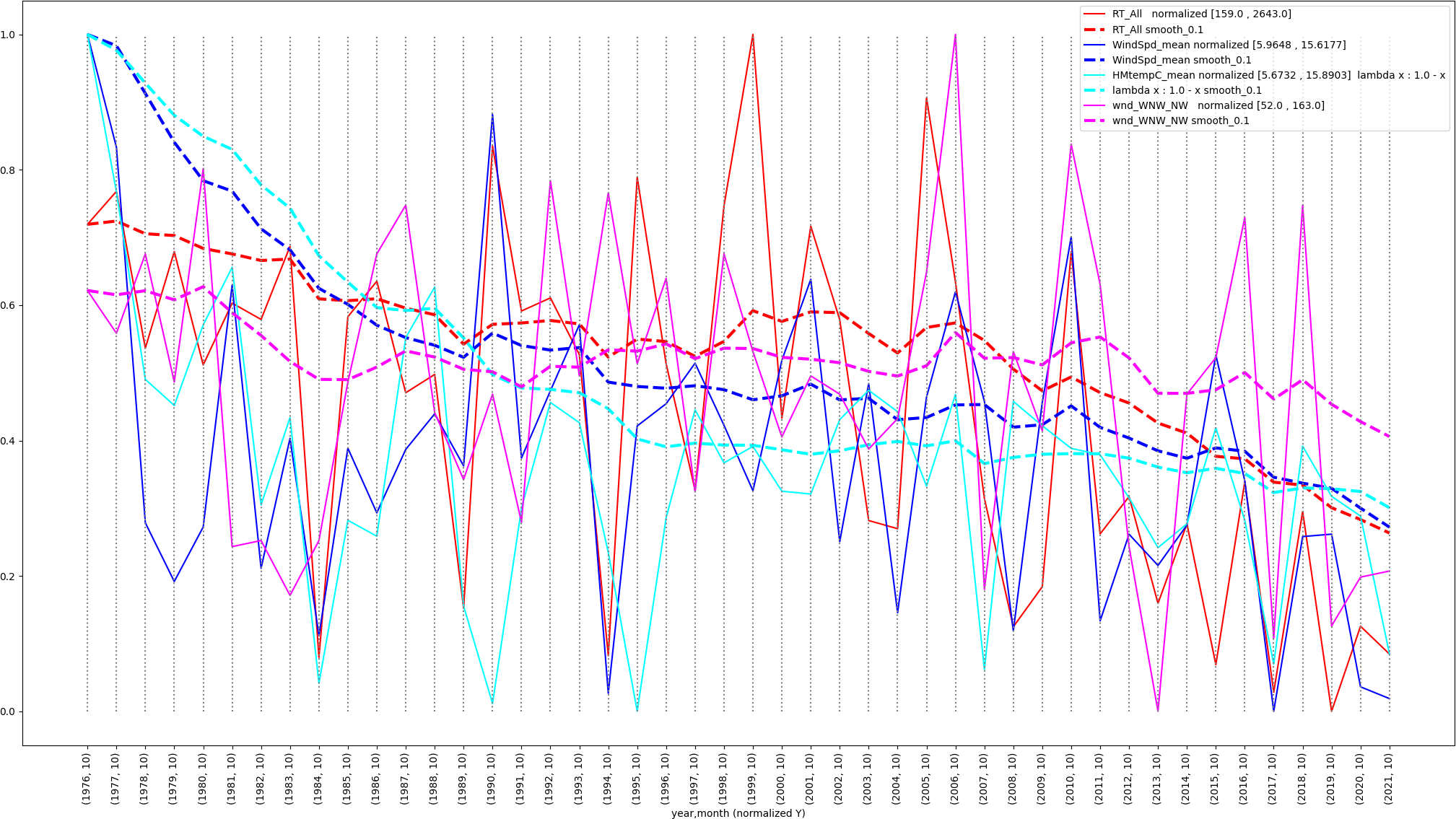
Here is Figure 4 from the summer 2023 analysis of red-tailed hawk declines in October 1976-2021.


Figure 1: Summer 2023 Figure 4 visualization of RT_All counts via exponential smoothing with an alpha of 0.1

Here is the text that accompanies that graphic from the summer of 2023:

---

The range of red-tailed hawk counts in Figure 4 for October, [159, 2643], is much higher than [22, 208] for Figure 3 of September, a more statistically significant sample size.

Smoothed Linear Regression Model for October 1976 through 2021
RT_All_smooth =
      0.5387 * HMtempC_mean_smooth +
      1.1919 * WindSpd_mean_smooth +
     -0.3542
Correlation coefficient                  0.8431

Modeling 1990 through 2021 when the smoothed attribute slopes of Figure 4 roughly converge increases the CC about 9%. WindSpd_mean_smooth is the strongest contributing attribute in terms of its multiplier in the linear expression, with HMtempC_mean_smooth coming in second. Normalization puts all attributes on the same scale so that the multipliers are comparable.
 
Smoothed Linear Regression Model for October 1990 through 2021
RT_All_smooth =
      0.8032 * HMtempC_mean_smooth +
      1.6502 * WindSpd_mean_smooth +
      0.5137 * wnd_WNW_NW_smooth +
     -0.9813
Correlation coefficient                  0.9211

---

I have been concerned that my use of an alpha value of 0.1 may have under-valued short-term trends by flattening them out.
For each attribute in the above graph, the smoothed value = (alpha * the current value) + ((1.0-alpha) * the previous smoothed value)
    where alpha ranges between (0.0, 1.0). Figure 1 uses alpha = 0.1.
The exponentially smoothed dashed lines above show overall trends, but they may miss important short-term trends.

The current assignment generates and analyzes data illustrated in the next four figures, ordered by correlation coefficients (CCs).


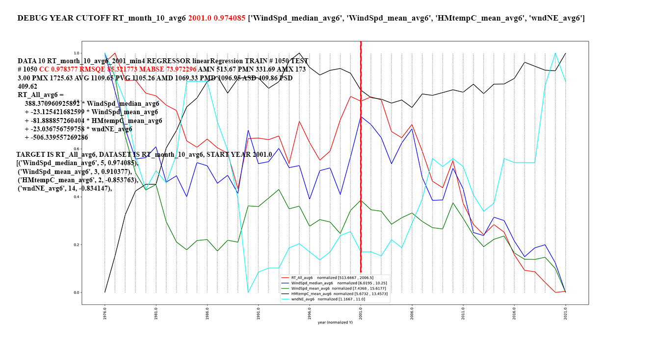
Figure 2: RT_All trends starting in 2001, the trend of the highest CCs for rolling average of 6 years per attribute.

The rolling average of avg6 means taking a 6-year rolling mean for each attribute except year and month.
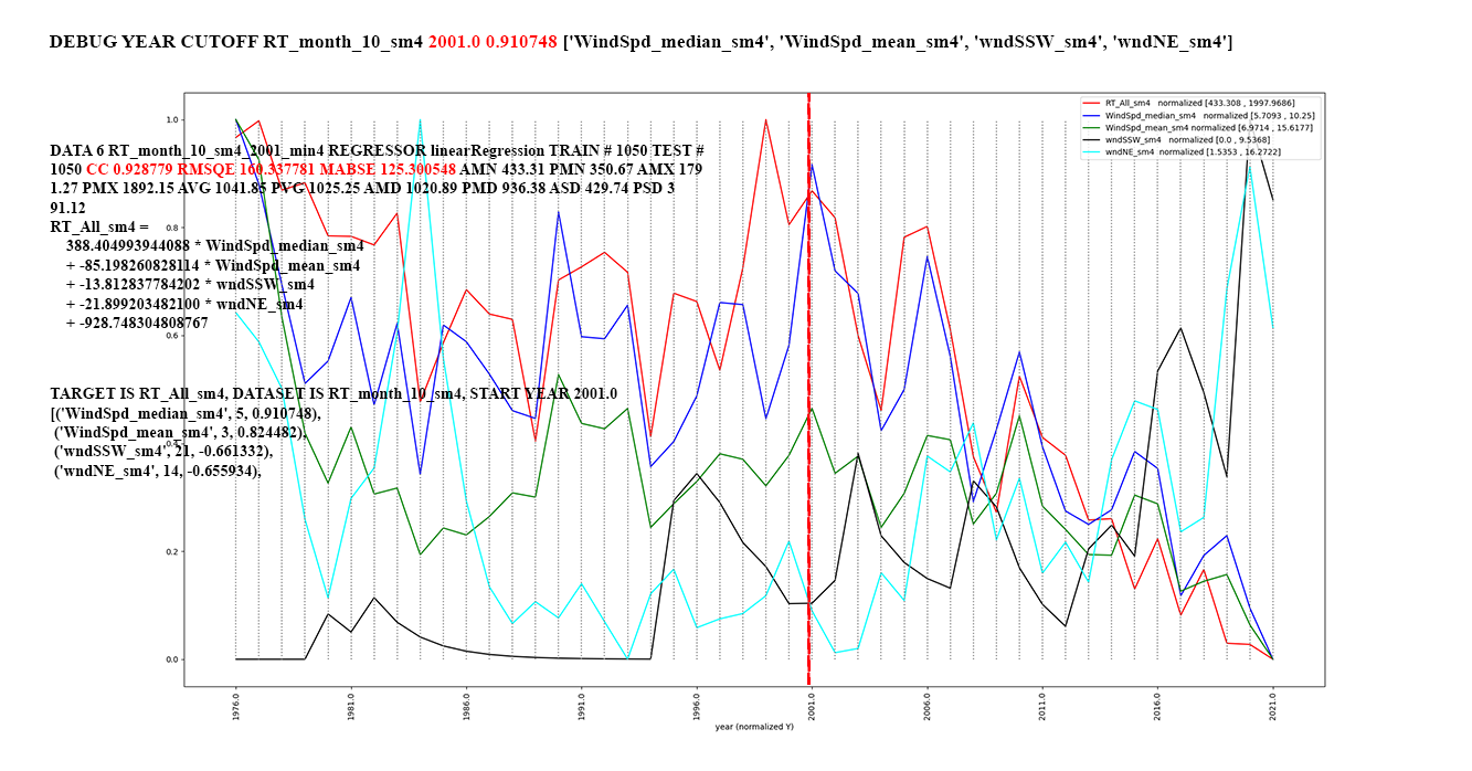
During the first 5 years the averaging function simply takes the mean of the available years to that point.

Figure 3: RT_All trends starting in 2001, the trend of the highest CCs for exponential smoothing with alpha=0.4.

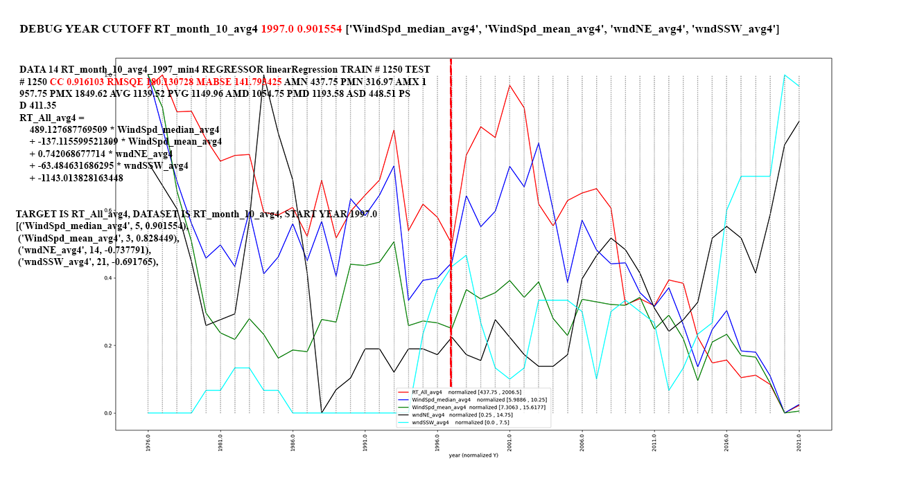
Alpha = 0.4 is higher that 0.1. Note how the smoothed attribute values track peaks and valleys more closely than in Figure 1.

Figure 4: RT_All trends starting in 1997, the trend of the highest CCs for rolling average of 4 years per attribute.

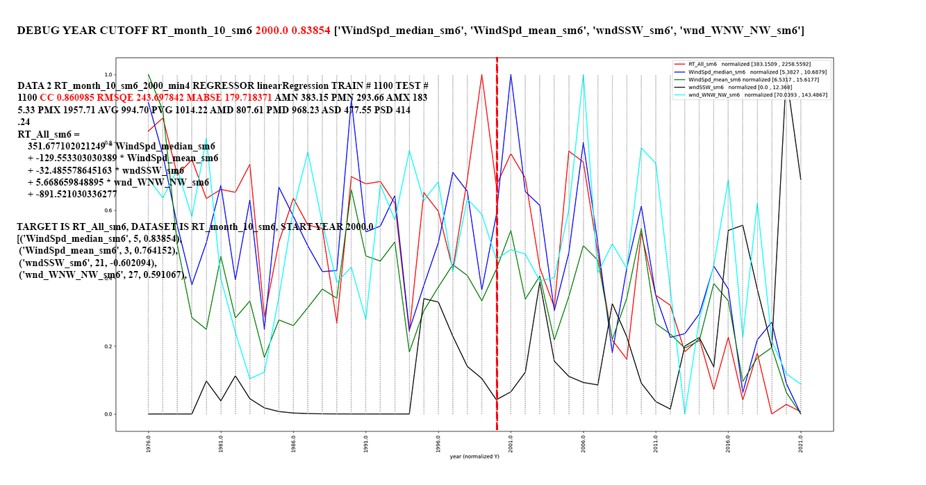
Figure 5: RT_All trends starting in 2000, the trend of the highest CCs for exponential smoothing with alpha=0.6.

We will go over the above graphs on November 20.

Please consult and complete the questions in README.txt before turning in Assignment 4.

60% of your points are for coding in STUDENT requirements of CSC523f23TimeSeriesAssn4_generator.py
and 40% are for answers in README.txt. Make sure to answer README.txt in your project directory. A missing
README.txt incurs a late charge.