CSC 523 - Advanced DataMine for Scientific Data
Science, Fall 2023, M 6-8:45 PM, Old Main 158.
SEE START OF CLASS
ZOOM RECORDING OF NOV. 6 TO CLARIFY
STUDENT 5, 7, & 8, referring to the data
visualization figures below "Addendum 11/4/2023".
Assignment 3 Specification, code is due by end of
Monday November 20 via make turnitin on acad or
mcgonagall. Perform the
following steps on acad or mcgonagall after logging into your
account via putty or ssh:
cd
# places you into your login directory mkdir DataMine
# all of your csc223 projects
go into this directory cd ./DataMine
# makes DataMine
your current working directory, it probably already exists cp
~parson/DataMine/CSC523f23AudioAssn3.problem.zip
CSC523f23AudioAssn3.problem.zip unzip CSC523f23AudioAssn3.problem.zip
# unzips your working copy of the project directory cd ./CSC523f23AudioAssn3
#
your project working directory
Perform all test execution on mcgonagall to avoid any
platform-dependent output differences.
All input and output data files in Assignment 2 are small and
reside in your project directory.
Here are the files of interest in this project directory.
There are a few you can ignore. Make
sure to answer README.txt in your project
directory. A missing README.txt incurs a
late charge.
CSC523f23AudioAssn3_generator.py # your work goes here,
analyzing correlation coefficients and kappa for
regressors
& classifiers
CSC523f23AudioAssn3_main.py #
Parson's handout code for building & testing
models that your generator above provides makefile
# the Linux make utility uses this script to direct testing
& data viz graphing actions makelib
# my library for
the makefile csc523fa2023AudioHarmonicData_32.csv.gz and AmplAvg128.csv.gz are
the two input data files. csc523fa2023AudioHarmonicData_32.csv.gz
has ordered attributes ampl1 and freq1, which are the
amplitude and frequency
of the fundamental frequency,
normalized to 1.0, and ampl2 and freq2 through ampl32
and freq32 are the fractional amplitudes
and multiples of ampl1 and freq1
respectively, as extracted by
extractAudioFreqARFF17Oct2023.py. The _32 refers to
aggregating 22050 discrete frequency
histograms from 0 through 22,050 cycles per second
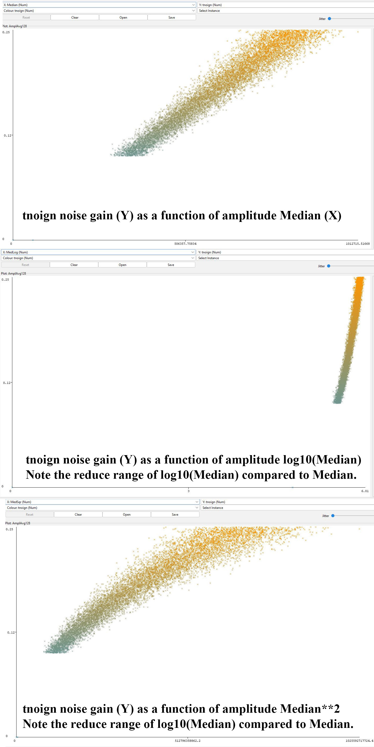
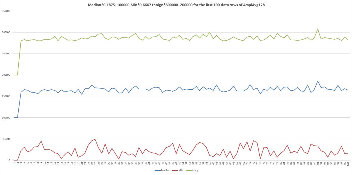
(hertz) into 32 histogram bin. AmplAvg128.csv.gz
aggregates all amplitudes of 128
histogram bins of the same data into these
attributes:
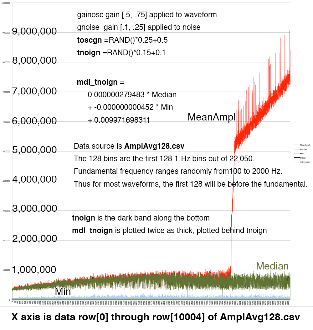
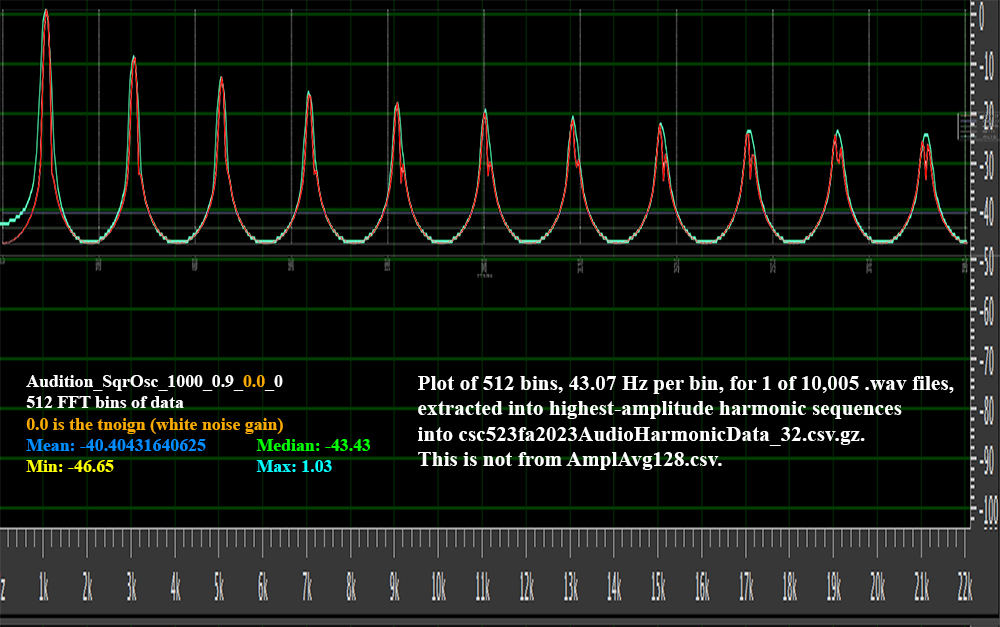
Figure 0: First 10 rows of 10,005 from
csc523fa2023AudioHarmonicData_32.csv.gz,
note the frequency
distributions of square etc. "A
square wave consists of a
fundamental sine wave (of the
same frequency as the square
wave) and odd harmonics of the
fundamental."
MeanAmpl mean of all
frequency domain amplitudes
Median
similar for
Median, Population Standard Deviation, Min,
and Max
PStdev
Min
Max
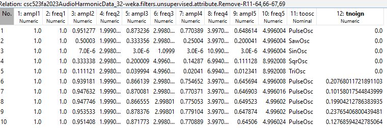
MeanLog log10() of
the above measures, compressing data as seen
in Figure 1 below
MedLog
SdLog
MinLog
MaxLog
MeanSqr
squaring (**2) the above
measures,
compressing data as
seen in Figure 1
below
MedSqr
SdSqr
MinSqr
MaxSqr
tnoign
white noise gain [0.1,
0.25] on a scale of [0.0, 1.0].
As
usual, make clean test tests your code and make
turnitin turns it into me by the due date.
There is the usual 10% per-day late change after the
deadline. make sure to turn in README.txt.
We will go over this Monday October 30 and at
least half of the November 6 class will be
work time.
Half of your points are for coding in STUDENT
requirements of CSC523f23AudioAssn3_generator.py
and half are answer in README.txt. Make sure to
answer README.txt in your project directory. A
missing
README.txt incurs a late charge.
*******************************************************************
# STUDENT 1: 20%, Read &
store data sets from CSV files.
# FOR all file names in
sorted(openFileSet)
# IF the file name
endswith '.gz' (use str.endswith(...))
# filehandle =
gzip.open(the file name, 'rt') # use 'rt'
# https://docs.python.org/3.7/library/gzip.html
# ELSE
# filehandle =
.open(the file name, 'r')
# filecsv =
csv.reader(filehandle)
# LOAD the data set
in filecsv into a list of rows, where each
# row is a list
of cells within that row, where each cell
# has been
translated via convert(cell) into a float if it
# is one, else
it remains a string. See def convert() above.
# This could be
a nested for loop or a nested list comprehension.
# IF the file name
startswith 'AmplAvg128.csv'
# Call
PrintCCstats(ccstats, file name, data set header
row[0],
#
remaining data set rows [1:], 'tnoign')
# FOR all data keys
in inputCSVmap.keys():
# IF
inputCSVmap[data key][0] == file name
#
inputCSVmap[data key][0] = data set, where row[0] is
the header
# IF
inputCSVmap[data key][1] == file name
#
inputCSVmap[data key][1] = data set, where row[1:]
is the data
# CLOSE THE
filehandle (last line within scope of FOR all file
names ...
# CLOSE ccstats AFTER (not
within) FOR all file names in sorted(...)
# # Comment: row[0]
of data set is header, row[1:] of data set is data
pass # STUDENT
1 code starts on the next line.
# STUDENT 2: 10%, Update
inputCSVmap[data key][4] with getData 6-tuple
# FOR all data keys in
inputCSVmap.keys():
# sixTuple =
getData(inputCSVmap[data key's][TRAININGDATA],
# inputCSVmap[data
key's][TESTNGDATA],
# inputCSVmap[data
key's][TARGET ATTRIBUTE NAME],
# inputCSVmap[data
key's][list of attributes to discard]
# inputCSVmap[datakey][4] =
sixTuple
pass # STUDENT
2 code starts on the next line.
# STUDENT 3: 10% Make shuffled
copy of the big 10K
# CREATE a variable
big10Kshuffled consisting of
# row[0] of
inputCSVmap['big10K'][TRAINING DATA] and a copy of
# row[1:] of
inputCSVmap['big10K'][TRAINING DATA] passed through
# shuffle() with
random_state=220223523
# CREATE a variable
big10Kshuffle6Tuple, passing big10Kshuffled as
# the first two
arguments (TRAINING and TESTING data) and the
#
inputCSVmap['big10K'][TARGET ATTRIBUTE NAME],
#
inputCSVmap['big10K'][list of attributes to discard]
as arguments
# to getData(),
storing its return 6-tuple in big10Kshuffle6Tuple
pass # STUDENT
3 code starts on the next line.
# STUDENT 4: 10% Make copy of
inputCSVmap['ampl'] with MEDIAN,MEAN,target
# RETRIEVE the header from
inputCSVmap['ampl'][0] row[0]
# RETRIEVE the target name from
inputCSVmap['ampl'][2]
# MAKE a new header list:
['Median', 'Min', target name]
# MAKE a NOT header list of every
attribute name in the retrieved header
# that is NOT in the
new header list
# Call
getData(inputCSVmap['ampl'][TRAINING DATA],
#
inputCSVmap['ampl'][TESTING DATA], target name,
# NOT header list to
discard) store returned 6-tuple from getData() in
#
amplMedianMin6Tuple.
# REMAINING STUDENT 5
through 9 WORK IS IN README.txt.
pass # STUDENT
4 code starts on the next line.
The other half are answers in REDAME.txt:
SEE START OF CLASS ZOOM
RECORDING OF NOV. 6 TO CLARIFY STUDENT 5, 7,
& 8.
STUDENT 5 10%: Consult the correlation coefficients
for tnoign from
AmplAvg128.csv.gz in file
CSC523f23AudioCCs.ref.
Consult these two decision tree structures in
CSC523f23AudioStructured.ref
DATA 5 ampl REGRESSOR decisionTreeRegressor TRAIN #
5002 TEST # 5003
CC 0.960595 RMSQE 0.012141 MABSE
0.009578 AMN 0.10 PMN 0.11
AMX 0.25 PMX 0.23 AVG 0.18 PVG
0.17 AMD 0.18 PMD 0.18 ASD 0.04 PSD 0.04
22 LINES IN REGRESSOR TREE
tnoign =
DECISION TREE PRINT OUT
DATA 6 amplMedianMin REGRESSOR decisionTreeRegressor
TRAIN # 5002 TEST # 5003
CC 0.960595 RMSQE 0.012141 MABSE
0.009578 AMN 0.10 PMN 0.11
AMX 0.25 PMX 0.23 AVG 0.18 PVG
0.17 AMD 0.18 PMD 0.18 ASD 0.04 PSD 0.04
22 LINES IN REGRESSOR TREE
tnoign =
DECISION TREE PRINT OUT
Note their respective correlation coeffcient values,
root mean squared error,
and mean absolute error measures. Also note this
model constructor from
CSC523f23AudioAssn3_generator.py:
decisionTreeRegressor =
DecisionTreeRegressor(min_samples_split=1000,
random_state=220223523) https://scikit-learn.org/stable/modules/generated/sklearn.tree.DecisionTreeRegressor.html
How do the attributes in these decsion trees in
CSC523f23AudioStructured.ref
relate to the CCs of attributes in
CSC523f23AudioCCs.ref? What effect
does the reduction of attributes down to [MEDIAN,
MIN, tnoign] have
on the CC and error measures of DATA 6's tree? Why
do you think that is?
STUDENT ANSWER:
*******************************************************************
STUDENT 6 10%: What effect does the parameter
min_samples_split=1000
in the DecisionTreeRegressor constructor call of
STUDENT 5 have on
the tree structures in STUDENT 5? EXPERIMENT by
setting
min_samples_split=2, which is its default, and
examining the resulting
DATA 5 and DATA 6 CCs and tree structures in
CSC523f23AudioStructured.tmp
(ignore the diff). Do the correlation coeffcients
improve or degrade in
going to a deeper tree? Does human intelligibility
improve or degrade
in going to a deeper tree? (Make sure to restore
min_samples_split=1000
and get "make test" to pass again.)
STUDENT ANSWER:
******************************************************************* SEE START OF
CLASS ZOOM RECORDING OF NOV. 6
TO CLARIFY STUDENT 5, 7, &
8. STUDENT
7 10%: Examine Figure 1 in the assignment handout
and
the Data 2 and 3 CCs and Linear Regression formulas
of
CSC523f23AudioStructured.ref. Why do you think the
DATA 3 tree has a CC
that is within 1.2% of Data 2's value, given the
loss of most of the
attributes? How does going from the linear
regression formula of
DATA 2 to DATA 3 relate to MDL (Minimum Decsription
Length), given
the fact that the reduction in CC accuracy is much
less than my 10%
threshold for MDL?
In [2]: (0.974525-0.963444)/0.974525
Out[2]: 0.01137066776121701
Consulting CSC523f23AudioCCs.ref may also help with
this answer.
Make sure to refer to Figure 1 in your answer.
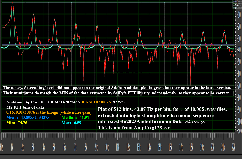
The first five in this question are reference
waveforms with 0.0
tnoign whitenoise gain, while the last five have
tnoign values ranging
from 0.139453694281 to 0.18926762076_534545. Given
the difference
in these waveform plots between tnoign=0.0 and
tnoign in the range
0.1 to 0.25, why do you think Median and Min are
more closely correlated
with tnoign level than Mean, Standard Deviation,
Min, or Max?
Put another way, why is CSC523f23AudioCCs.ref
ordered the
way it is? Why do Median and Min sit at the top of
its CC ordering?
STUDENT ANSWER:
*******************************************************************
STUDENT 9 10%: CSC523f23AudioAssn3.sorted.ref shows
the following:
DATA 17 big10Kshuffled CLASSIFIER
decisionTreeClassifier
TRAIN # 5002 TEST # 500 3 kappa
1.000000 Correct 5003 %correct 1.000000
DATA 16 big10K CLASSIFIER decisionTreeClassifier
TRAIN # 5002 TEST # 5003 kappa
0.375562 Correct 3003 %correct 0.600240
Why does DATA 17 big10Kshuffled have a kappa of
1.000000 while
DATA 16 big10K have a kappa of only 0.375562 for
classifying toosc
(type of signal oscillator), given the fact that
they use the same data?
Your answer must include WHY the difference in these
two datasets had
this effect on kappa, and not just what your code
did to transform the data.
Is giving a non-uniform,
monotonically increasing
distribution of frequencies for
the last 833 SqrOsc below.
Signal and white noise gain from
random.uniform appears to be
fluctuating uniformly.