CSC 223 -
Python for Scientific Programming & Data Manipulation,
Fall 2023, TuTh 4:30-5:45 PM, Old Main 159
Notes on Pandas. We will use Pandas primarily
for relational data manipulation.
Links to Pandas Series, pre-DataFrame, Relational
Operation discussions below.
In [1]: import
numpy as np
In [2]: import pandas as pd
SERIES. A Pandas Series is a 1D
column of typed, indexed data.
The motivation for typed data is efficiency of
storage & manipulation.
In [6]: seq1 = pd.Series(range(0,34,3))
In [7]: seq1
Out[7]:
0 0
1 3
2 6
3 9
4 12
5 15
6 18
7 21
8 24
9 27
10 30
11 33
dtype: int64
In [8]: type(seq1)
Out[8]: pandas.core.series.Series
In [9]:
seq2 = pd.Series(i**2 for i in range(0,34,3))
In [10]: seq2
Out[10]:
0 0
1 9
2 36
3 81
4 144
5 225
6 324
7 441
8 576
9 729
10 900
11 1089
dtype: int64
In [14]: type(seq1[0])
Out[14]: numpy.int64
In [19]: seq3 = seq1 + seq2 # adds respective
elements
In [20]: seq3
Out[20]:
0 0
1 12
2 42
3 90
4 156
5 240
6 342
7 462
8 600
9 756
10 930
11 1122
dtype: int64
An index can be a string, giving an effect similar to a
Python dict.
In [23]: seq4 = pd.Series([25, 20, 20, 20],
...: index=['csc223.010', 'csc220.010',
'csc220.020', 'csc532.401'],
...: name='Parson Fall 2023 courses'
...: )
In [24]: seq4
Out[24]:
csc223.010 25
csc220.010 20
csc220.020 20
csc532.401 20
Name: Parson Fall 2023 courses, dtype: int64
In [26]: dict = {'a': 1, 'b':22, 'c':33}
In [27]: pdmap = pd.Series(dict)
In [28]: pdmap
Out[28]:
a 1
b 22
c 33
dtype: int64
In [32]: type(pdmap['b'])
Out[32]: numpy.int64
In [37]: pdmap.keys()
Out[37]: Index(['a', 'b', 'c'], dtype='object')
In [38]: pdmap.values
Out[38]: array([ 1, 22, 33])
In [39]: list(pdmap.keys()) # Convert to
Python list type.
Out[39]: ['a', 'b', 'c']
In [40]: list(pdmap.values)
Out[40]: [1, 22, 33]
In [42]: seq1.keys()
Out[42]: RangeIndex(start=0, stop=12, step=1)
In [43]: seq1.values
Out[43]: array([ 0, 3, 6, 9, 12, 15, 18, 21,
24, 27, 30, 33])
Missing numeric data translates to floating point NOT A
NUMBER, a.k.a. np.nan or NaN.
NaN
represents missing data or undefined data such as N
divided by 0.
Numpy also supports np.inf and -np.inf for positive &
negative infinities.
In [52]: seq9 = pd.Series([1, 2, None, 3])
In [53]: seq9
Out[53]:
0 1.0
1 2.0
2 NaN
3 3.0
dtype: float64
In [54]: quotient = 10 / 0
---------------------------------------------------------------------------
ZeroDivisionError
Traceback (most recent call last)
<ipython-input-54-5f06513a6ce0> in <module>
----> 1 quotient = 10 / 0
ZeroDivisionError: division by zero
In [55]: try:
...: quotient =
10 / 0
...: except Exception:
...: quotient =
np.nan
...:
In [56]: quotient
Out[56]: nan
In [57]: try:
...: quotient =
10 / 2
...: except Exception:
...: quotient =
np.nan
...:
In [58]: quotient
Out[58]: 5.0
There is support for missing int values using a
non-standard approach via dtype coercion.
In [59]: seq10 = pd.Series([1, 2, None, 3], dtype='Int64')
In [60]: seq10
Out[60]:
0 1
1 2
2 <NA>
3 3
dtype: Int64
In [61]: seq10[2]
Out[61]: <NA>
In [62]: type(seq10[2])
Out[62]: pandas._libs.missing.NAType
Series also support set-like categorical data via
dtype='category'.
Categorical data (e.g., 'happy', 'sad', 'bored') are used in
machine learning classification.
In [66]: seq11 = pd.Series(['a', 'c', 'd', 'a'])
In [67]: seq11
Out[67]:
0 a
1 c
2 d
3 a
dtype: object
In [68]: seq11 = pd.Series(['a', 'c', 'd', 'a'],
dtype='category')
In [69]: seq11
Out[69]:
0 a
1 c
2 d
3 a
dtype: category
Categories (3, object): [a, c, d]
Series support functions that aggregate data into scalars.
Here are a few.
In [80]: seq2
Out[80]:
0 0
1 9
2 36
3 81
4 144
5 225
6 324
7 441
8 576
9 729
10 900
11 1089
dtype: int64
In [81]: seq2.mean()
Out[81]: 379.5
In [82]: seq2.median()
Out[82]: 274.5
In [83]: (225+324)/2
Out[83]: 274.5
In [84]: seq2.min()
Out[84]: 0
In [85]: seq2.max()
Out[85]: 1089
In [86]: seq2.std() # Return sample
standard deviation.
Out[86]: 370.46052421276954
To find the index of a value (ugly, isn't it?):
In [93]: seq2[seq2 == 441].index[0]
Out[93]: 7
PRE_DATAFRAMES.
A Pandas DataFrame is a 2D sequence of 1D columns of typed,
indexed data.
It is great for saving storage of typed columns and
reducing columns of data.
It stinks at row-major data processing of relations,
e.g., a database row-oriented select.
Based
on the book I am leaning on, DataFrame is not
geared for row-oriented data manipulation:
"If you think of a database as row oriented, the
interface will feel wrong. Many tabular data structures
are row oriented.
Perhaps this is due to spreadsheets and CSV files dealt
with on a row by row basis." Chapter 16 Dataframes.
Parson: No, row orientation is required by many
datasets. Suppose you are trying to analyze dissolved
oxygen levels in a USGS stream sample as a function of
pH and temperature measures at the same time.
Furthermore, suppose you are creating derived attributes
-- new columns of data -- as a function of
other attributes in each row. Column orientation may be
fine for deriving time-series columns as a function
of limited numbers of columns (e.g., temperature change
per unit time as a function of successive time steps)
or aggregating a column's mean, etc., as demoed for
Series above, but for many applications, organizing
memory in columns is inefficient. The real selling point
is that a given column usually has a fixed data type
as demoed with Series above, reducing per-cell memory
requirements and value accessing compared
to Python's built-in heterogeneous data types via
pointers to type-tagged objects. However, Numpy scalars
and pandas scalars still use pointers to underlying C
types.
In [3]: i = 3
In [4]: type(i)
Out[4]: int
In [5]: isinstance(i, object)
Out[5]: True
In [6]: i = 3.0
In [7]: type(i)
Out[7]: float
In [8]: isinstance(i, object)
Out[8]: True
In [9]: i = None
In [10]: type(i)
Out[10]: NoneType
In [11]: isinstance(i, object)
Out[11]: True
In [12]: i = np.int64(3)
In [13]: type(i)
Out[13]: numpy.int64
In [14]: isinstance(i, object)
Out[14]: True
In [15]: i = np.float64(3)
In [16]: type(i)
Out[16]: numpy.float64
In [17]: isinstance(i, object)
Out[17]: True
In [18]: iarray = np.array([1, 2, 3, 4, 5])
In [20]: type(iarray)
Out[20]: numpy.ndarray
In [21]: type(iarray[0])
Out[21]: numpy.int32
In [22]: isinstance(iarray[0], object)
Out[22]: True
In [23]: iarray = pd.Series([1, 2, 3, 4, 5])
In [24]: type(iarray[0])
Out[24]: numpy.int64
In [25]: isinstance(iarray[0], object)
Out[25]: True
Numpy arrays also require every element in a row to be
the same datatype.
In [99]: npa1 = np.array(seq1)
In [100]: npa2 = np.array(seq2)
In [101]: npa1
Out[101]: array([ 0, 3, 6, 9, 12, 15,
18, 21, 24, 27, 30, 33])
In [102]: type(npa1[0])
Out[102]: numpy.int64
In [108]: npa2
Out[108]:
array([ 0, 9,
36, 81, 144, 225,
324, 441, 576, 729, 900, 1089])
In [106]: npa3 = [[npa1[index] , npa2[index]] for
index in range(0,len(npa1))]
In [107]: npa3
Out[107]:
[[0, 0],
[3, 9],
[6, 36],
[9, 81],
[12, 144],
[15, 225],
[18, 324],
[21, 441],
[24, 576],
[27, 729],
[30, 900],
[33, 1089]]
In [109]: npa4 = [[npa3[index] + npa3[index]] for
index in range(0,len(npa3))]
# Above command is a database join over the row
number.
In [110]: npa4
Out[110]:
[[[0, 0, 0, 0]],
[[3, 9, 3, 9]],
[[6, 36, 6, 36]],
[[9, 81, 9, 81]],
[[12, 144, 12, 144]],
[[15, 225, 15, 225]],
[[18, 324, 18, 324]],
[[21, 441, 21, 441]],
[[24, 576, 24, 576]],
[[27, 729, 27, 729]],
[[30, 900, 30, 900]],
[[33, 1089, 33, 1089]]]
More from the
book I am leaning on :
"Columns of a single type can be
compressed easily. Performing analysis on a
column requires
loading only that column, whereas a
row-oriented database would require reading
the complete
database to access an entire column."
Parson: Yes, and performing per-row
analysis requires loading only that row.
"When
your only tool is a hammer, everything
looks like a nail."
Python lists are implemented as contiguous
machine-level arrays, so if an
application
uses good locality-of-reference -- finish
the work in the current row or couple of
rows
before going onto the next -- then operating
system demand paging can page out rows
not currently being accessed.
Even better, use csv.reader, filter, and other lazy
generators to load & process rows when needed.
$ pwd
/home/kutztown.edu/parson/Scripting/pandas
$ ls -l
total 269740
-rw-r--r--. 2 parson domain users 276211811 Jun
7 2022 weatherData_2021_NOAA.csv
After doing the following:
$ python
Python 3.7.7 (default, May 11 2020, 11:42:40)
[GCC 4.8.5 20150623 (Red Hat 4.8.5-39)] on linux
Type "help", "copyright", "credits" or "license" for
more information.
>>> import csv
>>> bigfile =
open('weatherData_2021_NOAA.csv', 'r')
>>> bigcsv = csv.reader(bigfile)
This python process shows 35,629 4k pages of virtual
memory consumption:
ps -l 10705
F S UID PID PPID C
PRI NI ADDR SZ WCHAN
TTY TIME CMD
0 S 220822790 10705 5046 0 80 0 - 35629 poll_s
pts/0 0:00
/usr/local/bin/python3.7
After the following steps that load ALL of weatherData_2021_NOAA.csv into
virtual memory:
>>> header = bigcsv.__next__()
>>> len(header) # How many
columns?
133
>>> biglist = [row for row in
bigcsv] # Read in all rows
>>> len(biglist)
769683
>>> len(biglist) *
len(biglist[0]) # How many cells of
data
102367839
We get this jump in virtual memory size:
$ ps -l 10705
F S UID PID
PPID C PRI NI ADDR SZ WCHAN
TTY
TIME CMD
0 S 220822790 10705 5046 1 80 0 - 630684
poll_s
pts/0 0:12
/usr/local/bin/python3.7
Reading the entries CSV file into memory has
grown the process by 2,437,345,280
bytes
of virtual storage.
>>> (630684-35629) * 4096
2437345280
Now let's try the same approach while
simulating processing 1 row at a time:
$
python
Python 3.7.7 (default, May 11
2020, 11:42:40)
[GCC 4.8.5 20150623 (Red Hat
4.8.5-39)] on linux
Type "help", "copyright",
"credits" or "license" for more
information.
>>> import csv
>>> bigfile =
open('weatherData_2021_NOAA.csv',
'r')
>>> bigcsv =
csv.reader(bigfile)
We get the same starting size of
35,629 4k
virtual
pages.
$ ps -l 16836
F S UID
PID PPID C PRI
NI ADDR SZ WCHAN
TTY
TIME CMD
0 S 220822790 16836 5046 0
80 0 - 35629 poll_s
pts/0
0:00 /usr/local/bin/python3.7
Now
let's simulate loading and processing one
row at a time, with CSV buffering behind the
scenes.
>>> header = bigcsv.__next__()
>>> len(header) # How many
columns?
133
>>> count = 0
>>> for row in bigcsv:
... count += 1
...
>>> print(count)
769683
The process has not added even a single 4k
virtual page at this point. It had room to
spare:
F S UID PID
PPID C PRI NI ADDR SZ
WCHAN
TTY
TIME CMD
0 S 220822790 16836 5046 0 80 0 - 35629
poll_s
pts/0 0:05
/usr/local/bin/python3.7
Delayed ("lazy") evaluation of Python
generators including filter
and map
avoid over-filling memory.
So-called "eager
evaluation" does calculations or memory
loads as soon as possible.
Let's do some filtering!
$ cat countHours.py
import csv
f = open('weatherData_2021_NOAA.csv','r')
fcsv = csv.reader(f) #
Delayed reads of the file.
hdr = fcsv.__next__()
hourcol = hdr.index('HOUR')
print('hourcol', hourcol)
def filterFunc(row): # filter out rows with
hours outside 0..23
try:
hour =
int(row[hourcol].strip())
except: # could be
invalid line of data or non-int
hour =
-1 # invalid value
return (hour >= 0 and hour <= 23)
# filter delays execution until __next__() requests next
filter value.
filt = filter(filterFunc, fcsv) # Loop through 769,682
filtered rows.
count = {}
for h in range(0,24):
count[h] = 0
filt = filter(filterFunc, fcsv) # filter object does lazy
evaluation
try:
while True:
row =
filt.__next__()
hour =
int(row[hourcol].strip())
count[hour] += 1
except StopIteration: # __next__() aborts the loop
pass
print('count', count)
print('sum counts', sum(count.values()))
f.close()
$ python -i countHours.py
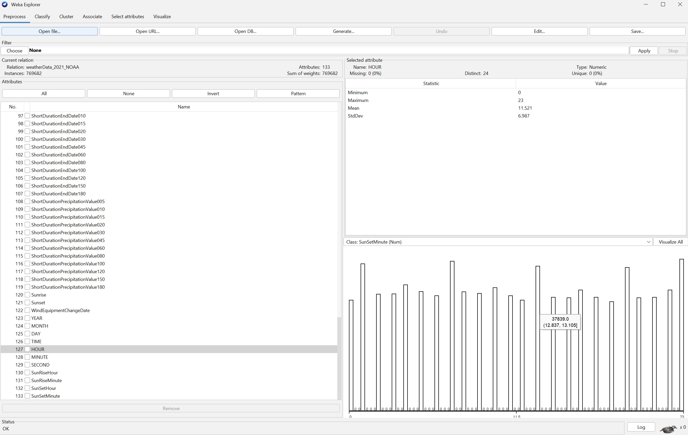
hourcol 126
count {0: 28971, 1: 38402, 2: 30440, 3: 30630, 4: 32960, 5:
31158, 6: 30042, 7: 39111, 8: 31067, 9: 30723, 10: 32250, 11:
30061, 12: 28952, 13: 37839, 14: 29710, 15: 29612, 16: 31630,
17: 29655, 18: 28536, 19: 37517, 20: 29532, 21: 29619, 22:
31611, 23: 39654}
sum counts 769682
>>>
$ ps -l 30773
F S UID PID PPID C
PRI NI ADDR SZ WCHAN
TTY TIME CMD
0 S 220822790 30773 21045 23 80 0 - 35609 poll_s
pts/2 0:06 /usr/local/bin/python3.7 -i
countHours.py
Seeming drop from 35629 pages. Later test run
with sleep(30) before and after yields 35613 pages.
CONCLUSION FOR 10/11/2023:
csv.reader and filter can be very efficient
for row processing without incurring costly storage overhead.
Some timing and memory expansion measurements for lazy
versus eager loading of data in memory.
$ python
Python 3.7.7 (default, May 11 2020, 11:42:40)
[GCC 4.8.5 20150623 (Red Hat 4.8.5-39)] on linux
Type "help", "copyright", "credits" or "license" for more
information.
>>> import csv
>>> import time
>>> f = open('weatherData_2021_NOAA.csv', 'r')
>>> fcsv = csv.reader(f)
>>> def filt(row): # filter function applied to
filter(filt,...)
... try:
...
return row[monthcol].strip() == '10' and row[daycol].strip()
==
'15'
... except: # usually missing
fields
...
return False
...
>>> hdr = fcsv.__next__() # get the header row
>>> monthcol = hdr.index('MONTH')
>>> daycol = hdr.index('DAY')
>>> def timedrun(f):
... # time iteration over f which is either
rows of data or a generator for rows
... global count
... count = 0
... before = time.time()
... cpubefore = time.process_time()
... for row in f:
...
count += 1
... after = time.time()
... cpuafter = time.process_time()
... print('count time CPUtime', count,
(after-before), (cpuafter-cpubefore))
...
>>> # measure memory size
$ ps -l 14011
F S UID PID PPID C
PRI NI ADDR SZ WCHAN
TTY TIME CMD
0 S 220822790 14011 31122 0 80 0 - 35700 poll_s
pts/0 0:00 /usr/local/bin/python3.7
>>> timedrun(filter(filt, fcsv))
count time CPUtime 2091 5.51302433013916 5.512656026
>>> count
2091
>>> f.seek(0)
0
>>> hdr2 = fcsv.__next__()
>>> hdr == hdr2 # verify hdr
True
>>> def myfilter(ffunc, data):
... # logically equivalent to built-in
filter(...) as a generator.
... for row in data:
...
if ffunc(row):
...
yield row
...
>>> timedrun(myfilter(filt, fcsv))
count time CPUtime 2091 5.491438865661621 5.491081708
>>> f.seek(0)
0
>>> hdr3 = fcsv.__next__()
>>> hdr == hdr3 # verify header
True
>>> # measure memory size
$ ps -l 14011
F S UID PID PPID C
PRI NI ADDR SZ WCHAN
TTY TIME CMD
0 S 220822790 14011 31122 2 80 0 - 35700 poll_s
pts/0 0:11 /usr/local/bin/python3.7
>>> before = time.time() ; cpubefore =
time.process_time() ; incoredata = [row f
or row in fcsv] ; after = time.time() ; cpuafter =
time.process_time()
>>> print('count time CPUtime', count,
(after-before), (cpuafter-cpubefore))
count time CPUtime 2091 12.025481462478638 12.024610784999998
>>> # measure memory size
$ ps -l 14011
F S UID PID PPID C
PRI NI ADDR SZ WCHAN
TTY TIME CMD
0 S 220822790 14011 31122 4 80 0 - 630684 poll_s
pts/0 0:23 /usr/local/bin/python3.7
>>> (630684 - 35700) * 4096
2437054464 # 2,437,054,464 bytes allocated to hold
incoredata
licd = len(incoredata) # number of rows
>>> licd
769683
>>> 2437054464 / (licd * len(incoredata[0])) # rows X
entries per row
23.806837067255078
>>> timedrun(filter(filt, incoredata))
count time CPUtime 2091 0.4378073215484619 0.4377831239999992
>>> timedrun(myfilter(filt, incoredata))
count time CPUtime 2091 0.4494149684906006 0.4493891189999992
NEXT UP Relational
Operations:
Python, Numpy arrays, and DataFrame for relational project
(columns), select (rows), and join (datasets).